PST Output Data Analysis Examples

The output data produced by the PST can be analysed using standard pulsar signal analysis tools like DSPSR and PSRCHIVE. It is also possible to analyse PST Voltage Recorder data using PyDADA.

The PST Team develops and maintains a Docker image with DSPSR and PSRCHIVE installed and ready for use. Instructions for launching and using this container can be found at SKA PST DSP Tools.

Example 1: square wave recorded in Digital PSI

In the following example, the output of a scan performed with the PST Voltage Recorder is assumed to be located in a folder named by the environment variable $DATA. Define

export IMAGE=harbor.skao.int/production/ska-pst-dspsr:0.2.0

and launch the ska-pst-dspsr docker container as follows

chmod a+r $HOME/.Xauthority
docker run -it -v $DATA:/mnt/data --net=host -e DISPLAY \
  -v ${HOME}/.Xauthority:/home/pst/.Xauthority $IMAGE bash

In the bash shell running in the docker container, change to the $DATA directory

cd /mnt/data

and confirm that all of the expected files are present. For example,

$ ls . data weights
.:
data  monitoring_stats  scan_completed  scan_configuration.json  ska-data-product.yaml  stat  weights

data:
2000-01-01-00:03:40_0000000000000000_000000.dada
2000-01-01-00:03:40_0000008068792320_000001.dada
2000-01-01-00:03:40_0000016137584640_000002.dada
2000-01-01-00:03:40_0000024206376960_000003.dada
2000-01-01-00:03:40_0000032275169280_000004.dada

weights:
2000-01-01-00:03:40_0000000000000000_000000.dada
2000-01-01-00:03:40_0000000068290560_000001.dada
2000-01-01-00:03:40_0000000136581120_000002.dada
2000-01-01-00:03:40_0000000204871680_000003.dada
2000-01-01-00:03:40_0000000273162240_000004.dada

You can check the various dimensions of the data with a command like

$ dada_edit data/2000-01-01-00:03:40_0000000000000000_000000.dada | grep ^N
NANT                2
NPOL                2
NBIT                16
NDIM                2
NSUBBAND            1
NCHAN               20736
NCHAN_OUT           20736

Three important header parameters are typically missing in the DADA file headers; these can be set with

dada_edit -c MODE=CAL */*.dada
dada_edit -c CALFREQ=50.23469650205761316872 */*.dada
dada_edit -c PFB_NCHAN=216 */*.dada

The CALFREQ parameter defines the frequency of the square wave in Hz, and PFB_NCHAN defines the number of fine frequency channels output by the second stage polyphase filter bank (PFB) for each coarse channel produced by the first stage PFB.

To prepare the data files for input to dspsr, it is necessary to create a “DUAL FILE” metadata file listing

ls data/*.dada > data.ls
ls weights/*.dada > weights.ls
cat > dual.ls << EOD
DUAL FILE:
data.ls
weights.ls
EOD

The average profile (phase-resolved average of the periodic modulating function) can be produced by running

$ dspsr dual.ls -T 1 -O folded
Disabling coherent dedispersion of non-pulsar signal
dspsr: blocksize=512 samples or 263.25 MB
unloading 1 seconds: folded

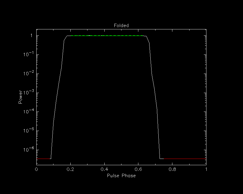
Note that this integrates only the first second of the recording. The output data file is named folded.ar and its contents can be plotted with

psrplot -x -pD -jF -c log=-1 folded.ar -D 1/xs \
  -c above:c="Folded" -c below:l=""

If successful, the above command will open an X11 window with the following plot

If unsuccessful (for example, if you see a message like PGPLOT /xw: cannot connect to X server []) then instead of plotting to an X11 window, you can plot directly to file by replacing -D 1/xs with another PGPLOT device like -D folded.gif/gif.

Note that the result looks modulated, but not very square. This is because the period of the square wave is 19.90656 milliseconds, and the sampling interval in the voltage time series output by the beam former is 207.36 microseconds. (Aside: the sampling interval can be queried with a command like the following.)

dada_edit -c TSAMP data/2000-01-01-00:03:40_0000000000000000_000000.dada

Therefore, the square wave is resolved by only 96 time samples. Furthermore, and more importantly, the voltages output by the beam former exhibit the sinc-like ringing of the impulse response function of the PFB used to channelize the second stage. Both the sampling interval and the width of this impulse response can be significantly reduced by inverting the second stage PFB.

PFB Inversion

First note that, in this example observation, NCHAN divided by PFB_NCHAN yields 96 coarse channels. (The relation between the number of coarse channels and the number of time samples per square wave period is coincidental.) To completely invert the second stage of channelization, run a command like the following

$ dspsr dual.ls -T 1 -IF 96:1024:128 -O inverted
Disabling coherent dedispersion of non-pulsar signal
dspsr: blocksize=352 samples or 279.938 MB
unloading 0.8 seconds: inverted

Note that only 0.8 seconds of data are integrated in the result output by dspsr, owing to edge effects that cause data loss at the beginning and end of the 1-second interval that is processed. Plotting the average profile with a command like

psrplot -x -pD -jF -c log=-1 inverted.ar -D 2/xs \
  -c above:c="PFB Inverted" -c below:l=""

should yield something like

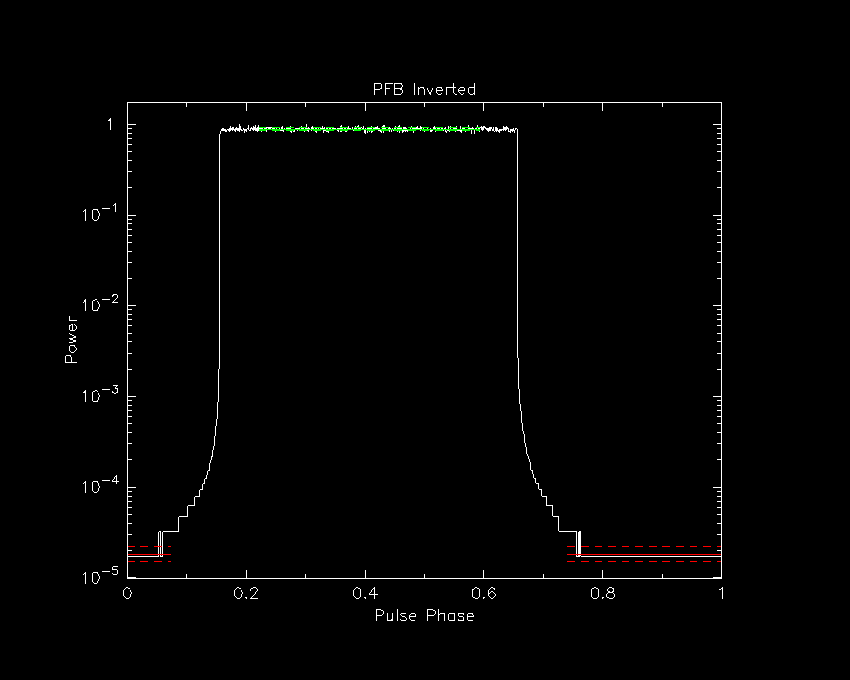
This looks a lot more square and sharp at the top. There remain some low-level artefacts (less than -30 dB) near the base of the square wave. These can be corrected by tapering the spectrum of each reconstructed coarse channel before performing the inverse FFT.

PFB Inversion with Spectral Tapering

To taper the spectrum of each coarse channel using a Hanning window, run

$ dspsr dual.ls -T 1 -IF 96:1024:128 -O inverted-tapered -f-taper hanning
Disabling coherent dedispersion of non-pulsar signal
dsp::InverseFilterbank::make_preparations prepare_spectral_apodization with DSB=1
dspsr: blocksize=352 samples or 279.938 MB
unloading 0.8 seconds: inverted-tapered

The resulting plot

psrplot -x -pD -jF -c log=-1 inverted-tapered.ar -D 3/xs \
  -c above:c="PFB Inverted and Hanning Tapered" -c below:l=""

should look like

The inversion artefacts are completely removed (nice!).

Example 2: pure tone recorded in Mid PSI

TO-DO