Ionospheric calibration

The ionospheric solver implemented in solve_ionosphere() fits low-order delay functions across the array aperture. Phase shifts are assumed to be proportional to the observed wavelength and to arise from variations in Total Electron Content (TEC) for different paths through the ionosphere. The solver uses Zernike polynomials in station position to model station-dependent \(\Delta\mbox{TEC}\) coefficients. As this parameterisation is independent of wavelength, all frequency channels and baselines can be used together to constrain a small number of parameters. As such, this approach can be more sensitive than direct antenna-based gain calibration.

While SKA-Low is large relative to relevant structure in the ionosphere, the clustered nature of stations in the array means that separate sets of Zernike polynomials can be used to model the different clusters, with relative shifts between clusters constrained in a single joint optimisation.

SKA-Low clusters

When calling solve_ionosphere() each station is assigned to one of these array “clusters” – a grouping of stations with their own set of Zernike basis functions. This can be controlled with the cluster_id parameter. The term “cluster” comes from the standard clusters in the Low array layout; a single cluster for the inner core of stations and an additional cluster for each grouping of six stations. However, the code is now more flexible and arbitrary groupings are possible. By default a single cluster will be generated for the whole array.

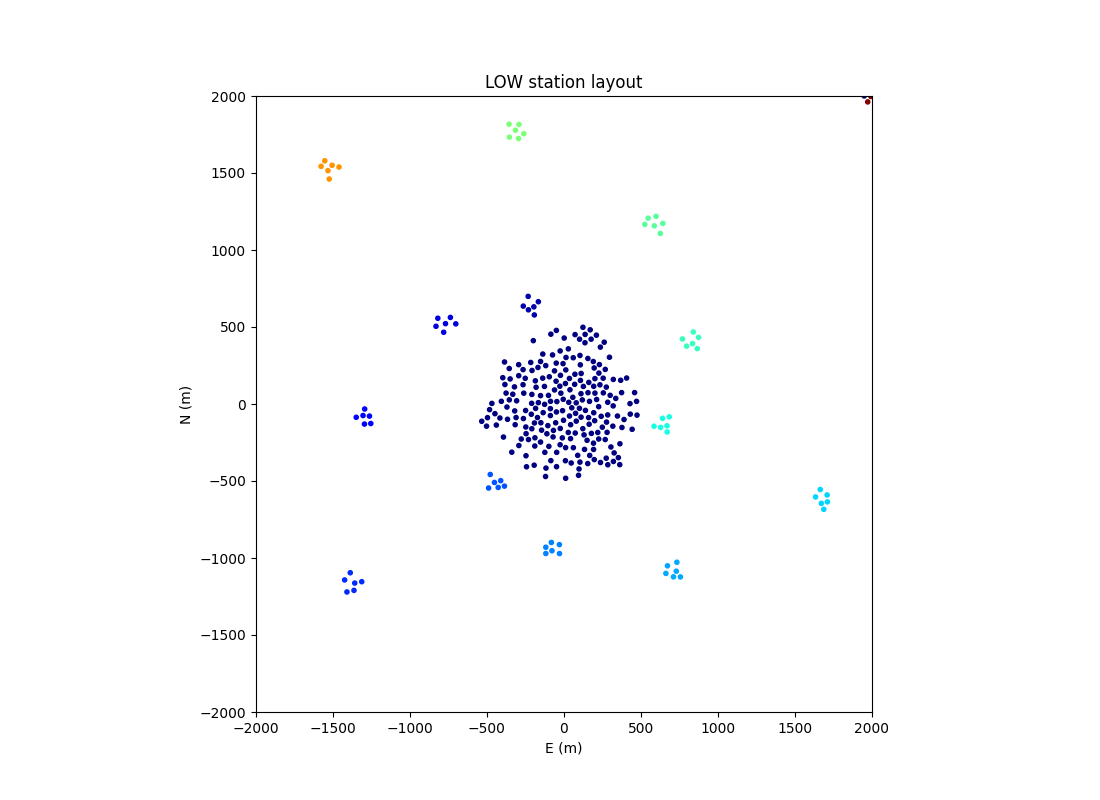
Inner part of the SKA-Low layout showing Low station clusters

While the underlying solver can use arbitrary basis functions, solve_ionosphere() is configured to use all Zernike polynomials with indices \(n+|m| \leq 6\) for cluster 0 (e.g. the SKA-Low core) and with indices \(n+|m| \leq 2\) for all other cluster. These limits can be controlled with the zernike_limit parameter. A subset of these functions is shown in the following figure.

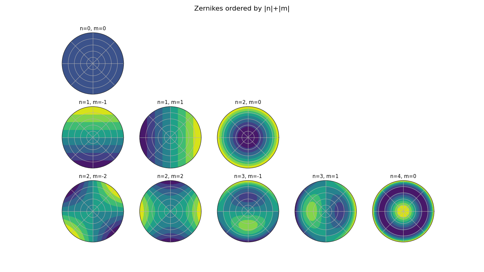
The first three Zernike polynomials represent a global, wavelength-dependent phase shift for the cluster (n=0, m=0), a wavelength-dependent northerly phase gradient across the cluster (n=1, m=-1), and a wavelength-dependent easterly phase gradient across the cluster (n=1, m=1).

Solving via normal equations

The visibility for stations j and k with an unknown ionospheric phase perturbation is modelled as

\[m_{jk} = m_{jk}^\prime \, e^{-i 2 \pi \lambda \left(\sum_p a_{f,p} f_p(x_j,y_j) - \sum_q a_{g,q} g_q(x_k,y_k)\right)}\]

where \(f_p(x,y)\) is the \(p^{th}\) Zernike polynomial at position x,y within the cluster containing station j, \(g_q(x,y)\) is the \(q^{th}\) polynomial for the cluster containing station k, and \(m_{jk}^\prime\) is the initial visibility model. Free parameter \(a_{f,p}\) is the fit solution for polynomial \(f_p(x,y)\). When j and k are in the same cluster the fit parameters are common, and the two first-order polynomials reduce to terms that are proportional to the separation of stations, which in the plane of the array are the u,v coordinates multiplied by wavelength. Thus the parameters describe a \(\lambda^2\)-dependent apparent angular shift for the sky model, as seen by this cluster. Higher-order terms tend to decorrelate the wavefront across the cluster.

As can be seen in the equation above, the unknown phase shifts are assumed to be constant across the sky model. Known direction-dependent effects can be incorporated into the model, but direction-dependent unknowns require multiple calls to the function, for example from a peel loop. The starting model, \(m_{jk}^\prime\), should include enough prior information about the sky, the array and perhaps the ionosphere that the unknowns are small and the exponential function can be linearised. For example, the model could include calibration factors from an initial direction-independent gain calibration step, or the model could be for an intermediate step in an iterative process. Subtracting such a linearised model from the observed visibilities leads to residuals of the form

\[r_{jk} = v_{jk} - m_{jk} \approx - i 2 \pi \lambda m_{jk} \left(\sum_p a_{f,p} f_p(x_j,y_j) - \sum_q a_{g,q} g_q(x_k,y_k)\right)\]

Derivatives with respect to the free parameters, -\(i 2 \pi \lambda m_{jk} f_p(x_j,y_j)\) for \(a_{f,p}\) and \(i 2 \pi \lambda m_{jk} f_q(x_j,y_j)\) for \(a_{g,q}\), can be added to a design matrix, A, with a column for each parameter and a row for each measurement, such that \(A \vec{a} = \vec{r}\), where \(\vec{a}\) and \(\vec{r}\) are vectors containing the unknown parameters and the residual visibilities, respectively. These can be solved via normal equations:

\[\begin{split}\vec{a} = (A^H W A)^{-1} A^H W \vec{r} \\\end{split}\]

where superscript H represents the Hermitian transpose and \(W\) is a diagonal matrix contaning sample weights. Multiplication by the complex conjugate model not only applies phase shifts and amplitude weighting that is appropriate for complicated calibration fields with multiple radio components and source morphology, it also ensures that it is only the real part of \(\vec{a}\) that is relevant.

Baseline and/or wavelength dependent weights can be incorporated into the normal equation \(W\) matrix via the weight data variable of the input Visibility dataset.

Optimisations

The solver forms and solves normal equations several times, each time improving the linear approximation until the system converges to a final set of solutions. The normal matrix is dominated by diagonal blocks, one for each set of cluster parameters, and it is often adequate to form and solve each block separately within each iteration of the convergence loop. While this may require more iterations to converge, it avoids rapid scaling with array size of both the number of operations and the memory usage. A similar approximation is used when solving for antenna-based gain terms in algorithms such as ANTSOL and StefCAL. Independent block matrices are enabled by setting parameter block_diagonal=True.