User Guide
Users control the Calculator via a web page interface, published at URL
http://example.com.
The observing configuration is described by setting values in the web interface. ‘Universal’ inputs required for all observing modes, such as the target position, are displayed in the upper part of the web page as shown in Fig. 1.
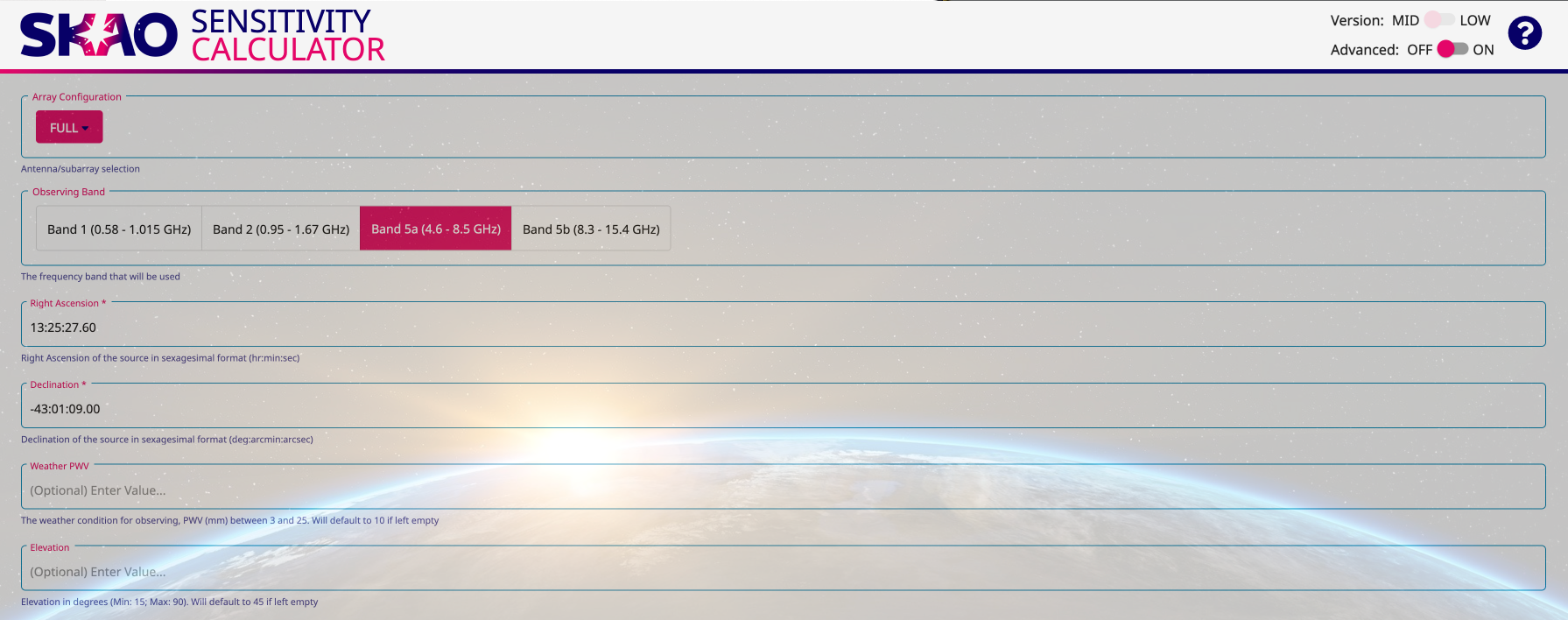
Figure 1 . Screenshot showing the ‘universal’ part of the Calculator page.
Configuration details that depend on observing mode are separated from the universal
inputs by tabs. The User can switch between modes by selecting either the Continuum
or Line tab, as shown in Fig. 2.
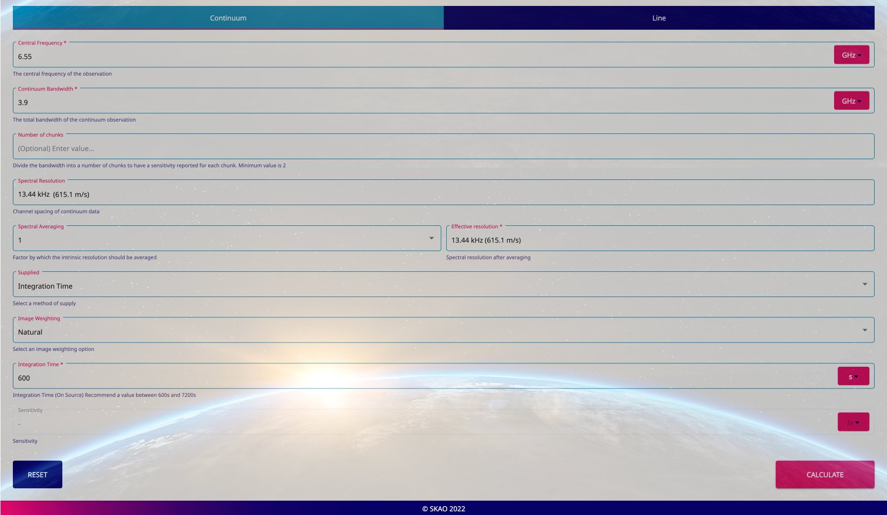
Figure 2 . Screenshot showing the tab for Continuum mode.
Once configured the Calculator can be used to either calculate the sensitivity for a given
on-source integration time, by selecting ‘Integration Time’ under the Supplied drop down,
entering the time and clicking calculate, or calculate the integration time required to
reach a given sensitivity, by selecting ‘Sensitivity’ under the Supplied drop down,
entering the sensitivity and clicking calculate. Fig. 3 shows an example report provided
to the user when this is done.
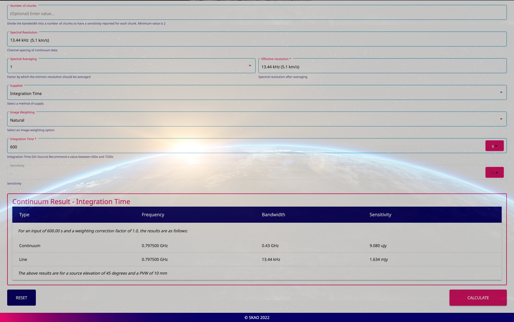
Figure 3 : Screenshot showing the report for the total continuum noise for a hypothetical observation. No PWV (Precipitable Water Vapour) or elevation angle were specified, and so the calculation is performed for default values.
Inputs
The calculator inputs can be categorised by the observing mode they fall under. Universal inputs are those that apply regardless of the selected observing mode.
Universal
Observing Band The selected band to use for the observation. For the “full” subarray the frequency ranges for the bands are:
Band 1: 0.58GHz - 1.015GHz
Band 2: 0.95GHz - 1.67GHz
Band 5a: 4.6GHz - 8.5GHz
Band 5b: 8.3GHz - 15.4GHz
Right Ascension and Declination The equatorial coordinates of the observed source. The sensitivity is calculated for the time at which the target reaches its maximum elevation, crossing the meridian.
Array Configuration Preset list of array configurations. Click on the tab to choose from:
SKA1 (133 x 15m): just the SKA1 antennas
full: all SKA1 and MeerKAT antennas
meerKAT: just the MeerKAT antennas
Not currently available:
custom: activates the nSKA and nMeer fields where the user can enter the number of SKA and MeerKAT antennas directly.
core
extended
Weather PWV If no value is set in the weather PWV (Precipitable Water Vapour) field then results will be given for the default value of 10mm, corresponding to “average” conditions. The PWV is used in the calculation of the atmospheric brightness temperature, \(T_{atm}\). Since \(T_{sys}\) is dependent on \(T_{sky}\) and therefore \(T_{atm}\) and the weather conditions, if the user decides to manually edit \(T_{sys}\) in ‘Advanced mode’, or any of the variables it depends on, the option to set the PWV will be removed.
Elevation The user can use this field to specify the elevation at which the target will be observed. If no value is set then a default of 45 degrees is assumed. If the given elevation is never reached by the target, then the target’s zenith elevation will be used. The actual elevation assumed for the sensitivity calculation is reported in the result table.
‘Advanced Mode’ Inputs By activating the ‘Advanced’ switch in the top right hand corner of the calculator, the user is given direct access to some of the parameters used in the sensitivity calculation, as shown in Fig. 4. The calculator front-end automatically enables/disables inputs to avoid conflicts as the user selects which one they want to edit. These are passed to the calculator back-end as hard-coded values which will override the calculated defaults.

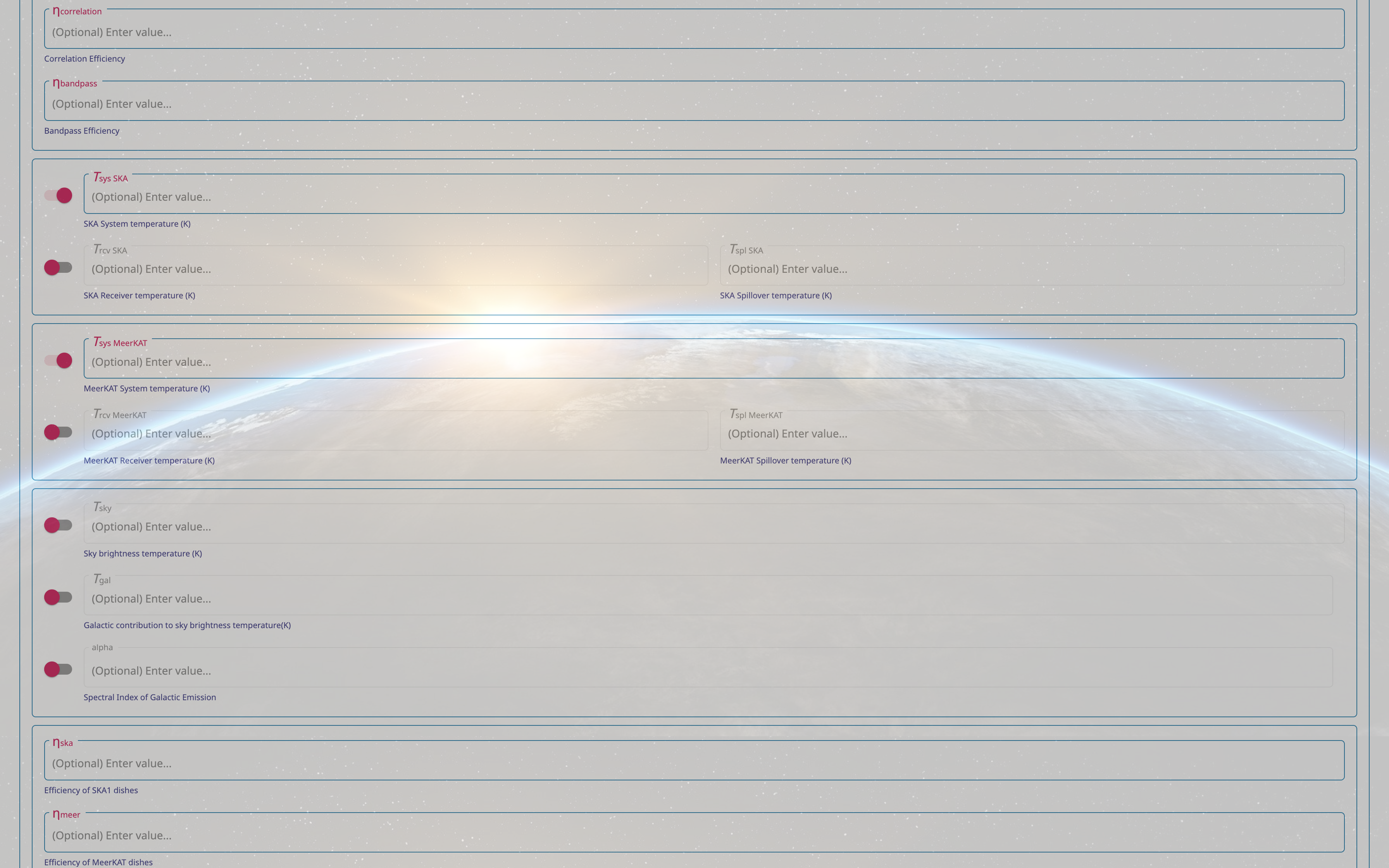
Figure 4 . Expanded view of an example use-case for the additional inputs on the ‘Advanced mode’ version of the calculator.
Continuum
Central Frequency The central frequency for the observation. Must be within the selected band.
Bandwidth The bandwidth for the observation. Must be fully contained within the selected band.
Number of chunks The user can select an integer number of chunks to split the bandwidth up into. If they do, the output report will show the sensitivity (or integration time) for each chunk.
Spectral Averaging The factor by which the intrinsic spectral resolution is averaged.
Supplied Drop down allowing the user to swap between integration time and sensitivity as the input (giving the other as the output).
Image Weighting The image weighting option to be used.
Integration Time The integration time of the observation. Used when calculating the sensitivity that observing for this amount of time will achieve.
Sensitivity The sensitivity for the observation. Used when calculating the integration time necessary to achieve this sensitivity.
Line
Zoom Frequency For each zoom, the user can input a frequency for that zoom. When a value is entered, the next zoom becomes enabled, allowing a value to be entered. It can however be left blank, and the calculation will only be done for zooms which have a set frequency. This way, the user can select how many zooms they want (up to a maximum, currently 4).
Zoom Bandwidth and Resolution For each zoom, the user can set a line resolution.
Supplied Drop down allowing the user to swap between integration time and sensitivity as the input (giving the other as the output).
Image Weighting The image weighting option to be used.
Integration Time The integration time of the observation. Used when calculating the sensitivity that observing for this amount of time will achieve.
Sensitivity The sensitivity for the observation. Used when calculating the integration time necessary to achieve this sensitivity.