SKA SDP Pointing Offset Calibration Pipeline
Introduction
This is a repository for the SDP pointing offset calibration pipeline. This repository reads Measurement Sets, optionally applies an RFI mask (pulled from ska-telmodel-data in real time) and/or select some frequency range of interest, and then fits the 2D Gaussian primary beams to the visibility or gain amplitudes. The fitted parameters are the Gaussian centre (provides the Cross-elevation and Elevation offsets), width (the fitted beamwidth), and height (in arbitrary units) and their uncertainties. These fitted parameters are then written to a text file and an HDF5 file created from a PointingTable for further analysis. The pipeline reads Measurement Sets using the Visibility class in ska-sdp-datamodels. When an RFI mask is applied and/or some frequency range is selected, the modified visibility is created with the ska-sdp-datamodels Visibility class for gain calibration (un-normalised G terms) or provides easy access to the visibilities and their associated parameters when fitting to them. These gains of each antenna are solved for using the gain solver in the ska-sdp-func-python library. The primary beam modelling and fitting is performed with scikits.fitting following the procedure used by the SARAO team for computing the pointing offsets for the MeerKAT array. The implementation of the pointing offset calibration pipeline follows the functionality diagram below
A list of the tools used in the pipeline are:
ska-sdp-datamodels: Provides function for reading measurement sets and converting the visibilities and all relevant tables to xarray object.
ska-sdp-func-python: Provides solver for calibrating for the complex gains of an antenna and function for converting antenna positions in Earth-Centred, Earth-Fixed to longitude, latitude and altitude coordinate system.
SciPy: Provides interpolation routine for aligning the actual pointings relative to the pointing calibrator and the visibility timestamps.
scikits.fitting: Provides routines for modelling the primary beam with a 2D Gaussian and fitting them to the gain amplitudes or visibilities.
katpoint: Used for constructing list of antenna information (location, diameter, etc) for easy use by the fitting routine.
NumPy: Used for manipulating arrays e.g, applying RFI masks.
Matplotlib: Provides routines for plotting e.g, Gaussian fitting plots, gain solutions, spectral, and temporal plots.
Pulling static RFI mask from SKA Telescope Model Data Repository
The repository hosting the channel-dependent RFI file in HDF5 format should first be set as an environment variable with an example below:
export SKA_TELMODEL_SOURCES=gitlab://gitlab.com/ska-telescope/ska-telmodel-data?yan-1618-add-rfi-model#tmdata
The path to the RFI file in the set branch above should be provided to the rfi_file argument. An example is provided below:
--rfi_file instrument/ska1_mid/static-rfi/rfi_mask.h5
The pipeline in real time pulls the RFI mask from the specified location and applies it to the visibilities. The pipeline is able to extract a smaller mask from the existing larger mask and apply to the visibilities if the frequency channels of the observation are fewer than the RFI mask in the Telescope Model Data Repository.
The Three-Dish Mode
To use fitting to the gain amplitudes functionality, at least three antennas are required for the gain calibration. Also, the pipeline requires all antennas to be moved simultaneously during a pointing offset calibration scan. The pointing offsets are calculated as follows similar to the description in the functionality diagram below

For each scan, the commanded pointings in AzEl coordinates are extracted from the TARGET column of the pointing sub-table or the commanded on-sky offsets in cross-elevation and elevation are extracted from the SOURCE_OFFSET column of the pointing sub-table.
When the commanded pointings in AzEl coordinates are used, their positions relative to the target are then computed with katpoint. For each scan, the target’s position is determined at the median of the pointings’ timestamps. The computed relative azimuth pointings are then converted to cross-elevation as the product of the relative azimuth and the cosine of the target’s elevation.
The un-normalised gains (G terms) for each scan are then solved for.
The primary beam modelled by a 2D Gaussian is fitted to the G terms from all the scans.
The fitted Gaussian centre are the cross-elevation and elevation offsets of interest.
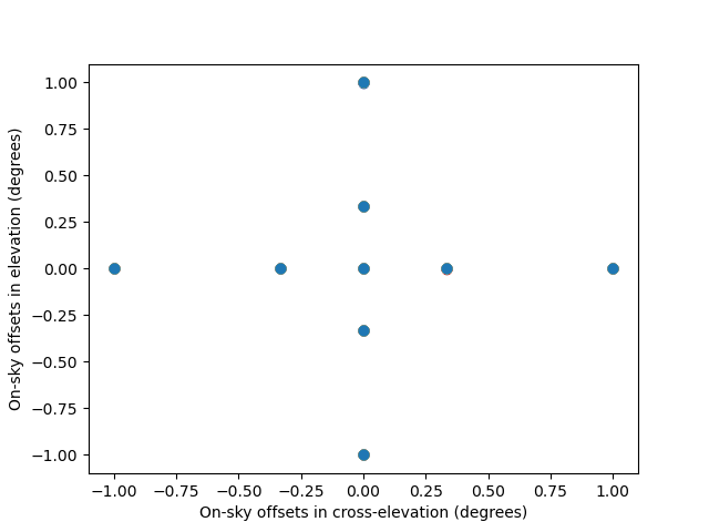
A sample nine-point scan with the MeerKAT array showing the on-sky offsets in cross-elevation and elevation is shown below

For a fit to be declared valid so the fitted offsets can be accepted, the pipeline ensures the following conditions are met:
The fitted Gaussian centre are physical i.e not NaNs.
The fitted Gaussian height is greater than zero.
The fitted width is within the user-provided tolerance of the expected width. The default is below 15% wider than the expected.
The fitting SNR is greater than zero.
The un-normalised gain amplitudes for each scan, over number of antennas with one curve per frequency chunk for the sample 9-point scan with the MeerKAT array is shown below.

The Gaussian fits in cross-elevation and elevation at each frequency chunk is shown below for antenna m000 from the sample 9-point scan with the MeerKAT array.

The weighted-average of the fitted parameters for all antennas from the sample nine-point scan with the MeerKAT array

The current pipeline can be executed as a CLI-based command line app. Please check the pointing_offset_cli page for usage instructions.
Installation Instructions
The package is installable via pip.
If you would like to view the source code or install from git, use:
git clone https://gitlab.com/ska-telescope/sdp/science-pipeline-workflows/ska-sdp-wflow-pointing-offset.git
Please ensure you have all the dependency packages installed. The installation is managed through poetry. Refer to their page for instructions.