PSS Candidate Viewer User Guide
The PSS candidate viewer is a command line application. The help section lists all possible options for the program.
>> candviewer -h

usage: candviewer [-h] [--makepdf] [--clean] [--force] [--show] -d DIR [--spcclext SPCCLEXT]
              [--filext FILEXT] [-s SUBBANDING_FACTOR] [--flatten] [--clip_percent CLIP_PERCENT]
              [--threshold_widths THRESHOLD_WIDTHS] [-t DOWNSAMPLING_FACTOR | --nsamp NSAMP]

PSS candidate viewer

options:
  -h, --help            show this help message and exit
  --makepdf             Combine candidate images into PDF
  --clean               Remove pngs from disk (if making PDF)
  --force               Skip confirmation prompt for --clean
  --show                Show interactive candidate plots as each one is processed

SPS candidate settings:
  -d DIR, --dir DIR     Path to SPS candidate directory
  --spcclext SPCCLEXT   SPS Candidate metadata extension (def=.spccl)
  --filext FILEXT       SPS candidate extension (def=.fil)
  -s SUBBANDING_FACTOR, --subbanding_factor SUBBANDING_FACTOR
                        Downsample in frequency by this factor (def=128)
  --flatten             Subtract the median bandpass from the dynamic spectrum before dedispersion
                        (def=False)
  --clip_percent CLIP_PERCENT
                        Symmetric percentile used to clip the colour scale of the plots (def=1)
  --threshold_widths THRESHOLD_WIDTHS
                        Number of pulse widths around the candidate timestamps to plot
  -t DOWNSAMPLING_FACTOR, --downsampling_factor DOWNSAMPLING_FACTOR
                        Downsample in time by this factor
  --nsamp NSAMP         Number of samples across pulse
Single pulse candidate viewer
The candviewer plots the output from a Cheetah SPS search pipeline, by reading the .spccl file and associate each candidate in it with the relevant .fil candidate data file. The candidate data files and the spccl list should be located in the same local directory. For example:
>> ls sps_beam1/
candidates.spccl
2012_03_14_00:00:00.fil
2012_03_14_00:00:05.fil
2012_03_14_00:00:11.fil
2012_03_14_00:00:17.fil
2012_03_14_00:00:23.fil
2012_03_14_00:00:29.fil
2012_03_14_00:00:34.fil
2012_03_14_00:00:40.fil
2012_03_14_00:00:46.fil

>> head sps_beam1/candidate.spccl
MJD(decimal days)           dm(dimensionless)                width(ms)               sigma                   label
56000.0002314993                     0.7                     0.256                   9.64                    0
56000.0005092771                     0.7                     0.256                   9.71                    0
56000.0006018667                     1.6                     0.512                   9.72                    0
56000.0006018697                     0.9                     0.064                   9.75                    0
56000.000138903                      1.6                     0.512                   9.8                     0
56000.0000463133                     1                       0.064                   9.88                    0
56000.0000463133                     1                       0.256                   9.89                    0
56000.0002314956                     1.4                     0.512                   9.92                    0
56000.0005092749                     0.9                     0.512                   9.94                    0
To plot those candidates with 8 samples across the pulse, and collect all the plots into one .pdf file, we can run:
>> candviewer -d sps_beam1/ --nsamp 8 --makepdf
This will create one .png image for each candidate in the candidate.spccl file, as well as append each plot into a file called candidate.pdf. The .png images will be uniquely named using the parameters of the relevant candidate, following the format <MJD>_DM<DM>_W<width>_SN<sigma>.png. The plots will be written to the same directory that holds the input candidate files.
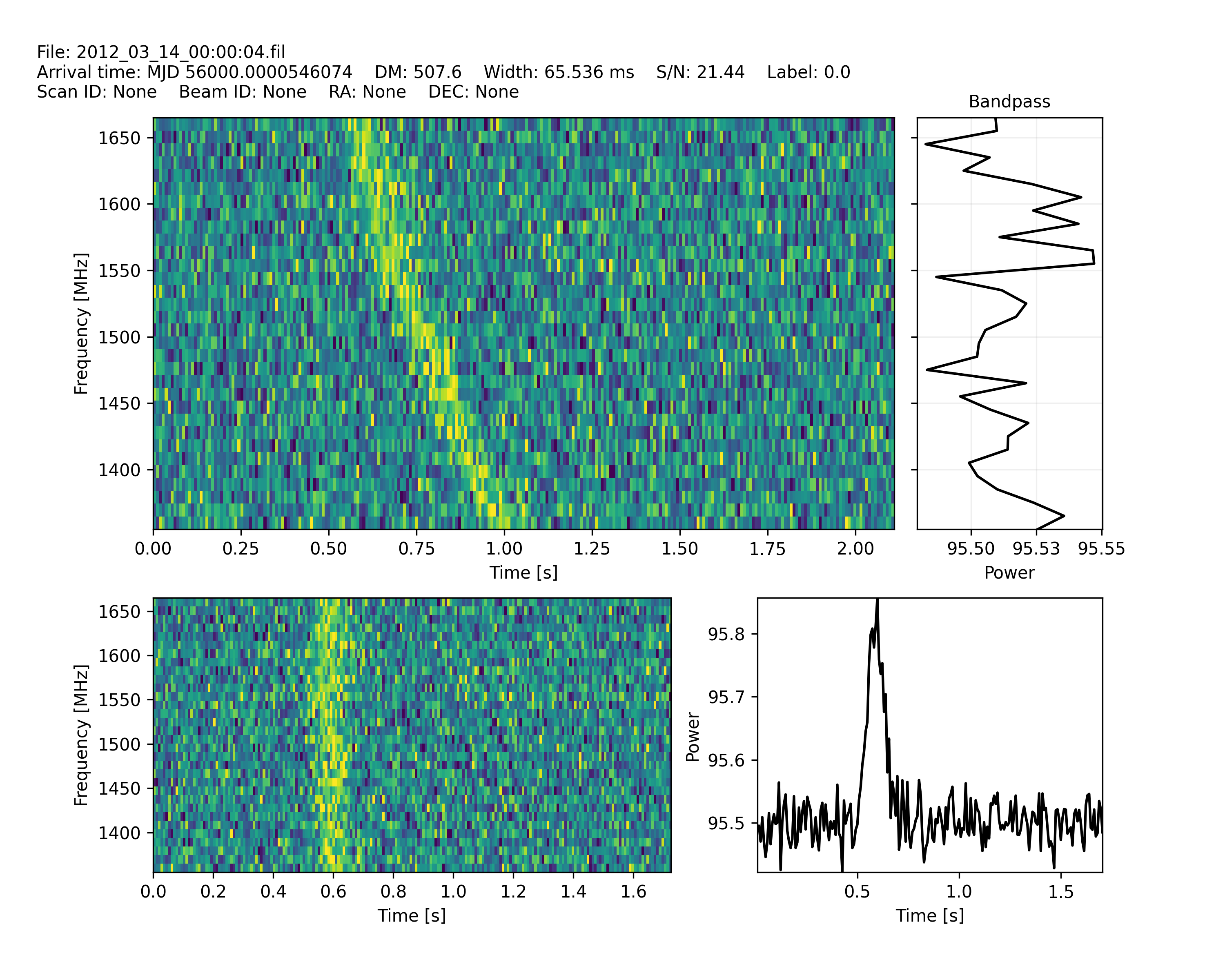
An example output plot, with a detected single pulse, is shown below. The top left panel shows the frequency band (in MHz) versus the integration time (in seconds) centered on the detected pulse, without dedispersion. The top right panel shows the integrated bandpass of that same time chunk. In the bottom left panel, the data has been dedispersed to the detected DM and again centered on the detected pulse. The bottom right panel shows the pulse profile power as a function of time, after dedipsersing the data and adding the frequency channels together.