MID Theoretical Background
Reference Documents
RD1 |
|
RD2 |
‘SKA1 Performance Assessment Report’ SKA-TEL-SKO-0001089 |
Applicable Documents
AD1 |
An improved source-subtracted and destriped 408 MHz all-sky map |
An overview of the theoretical performance of SKA Mid comprising SKA1 and MeerKAT dishes is given in RD1. A more detailed analysis is given in RD2 for an SKA Mid made up of only SKA1 dishes. We are grateful to Songlin Chen for help in navigating and understanding the documentation.
The Mid Sensitivity Calculator (SC) was originally implemented following the theoretical framework of RD1 but is moving to the more rigorous framework of RD2, though some details remain simplified.
Dish SEFD
The ‘system equivalent flux density’ (SEFD) for a single dish is the flux density of a source that produces a signal equal to the background power of the system:
where:
\(k\) is the Boltzmann constant so that \(kT_{sys}\) measures the power received from background emission and all other sources of unwanted signal within the system, that is \(T_{sys} = T_{spl} + T_{sky} + T_{rcv} + T_{cmb} + ...\)
\(\eta_A\) is the dish efficiency
\(A\) is the geometric dish area.
The 2 is there because a radio telescope measures only one polarization and it is assumed for this purpose that the other polarization has the same strength.
Array SEFD
SKA Mid is an interferometer that works by combining the signal from multiple dishes. There are 2 types of dishes involved, SKA1 and MeerKAT, with distinct characteristics. It can be shown, by adding up the signals from each baseline, that the array SEFD is given by:
where:
\(n_{\mathrm{SKA}}\) is the number of 15-m antennas
\(n_{\mathrm{MeerKAT}}\) is the number of 13.5-m antennas
\(SEFD_{\mathrm{SKA}}\) is the SEFD computed for an individual SKA antenna
\(SEFD_{\mathrm{MeerKAT}}\) is the SEFD computed for an individual MeerKAT antenna.
and the assumption has been made (?) that all baselines are equally efficient.
Array Sensitivity
The ‘sensitivity’ of a radio telescope is an overloaded term. For the purpose of the SC we define the sensitivity as the minimum detectable Stokes I flux (1 \(\sigma\)). This is equal to the noise on the background power, obtained using the radiometer equation \(\sigma = SEFD / \sqrt{2 B t}\), corrected for atmospheric absorption:
where:
\(\Delta S_{min}\) is the source flux density above the atmosphere
\(\eta_s\) is the efficiency factor of the interferometer
\(B\) is bandwidth
\(t\) is integration time
\(\tau_{atm}\) is the optical depth of the atmosphere towards the target
the formula applies to the centres of fields-of-view where the dish aperture response is unity.
Dependency Tree
The devil is in the detail of calculating \(T_{sys}\) and the efficiency factors \(\eta_A\) and \(\eta_s\). Fig.1 shows how these values depend on other factors that must be estimated.
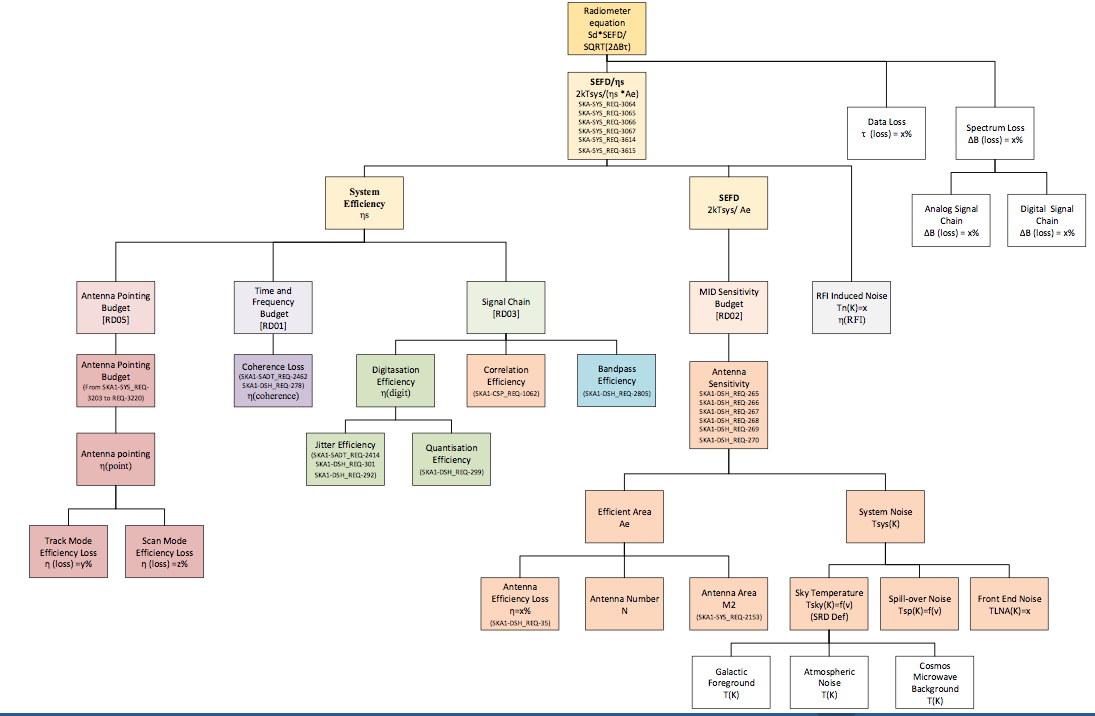
Figure 1 . The dependency tree for factors in the sensitivity calculation (from RD2).
The last implementation of the dependency tree in the sensitivity calculator is shown in the following image:
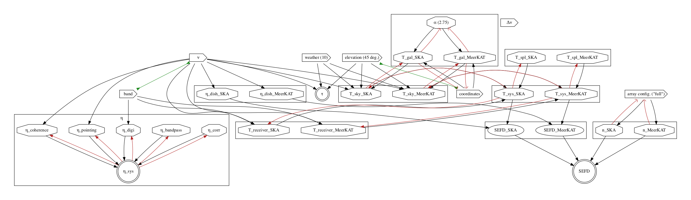
Figure 2 . The dependency tree for factors in the new implementation of the sensitivity calculator. Boxes with a triangular shape on the right are the fundamental inputs for the calculator. Variables that are in an octogon can be overridden in expert mode (see later). Variables in double circles are the result of the calculation through the dependencies. The black arrows mark dependencies. The green lines sanity and consistency checks. Red arrows indicate variables that are overridden if one of the downstream variables is set. If their arrow tip is circular it means that all the lines pointing to a variable (red arrows) must ve activated so that the variable is actually overridden.
The new implementation will be used from API v1 onwards.
System Temperature
The system temperature is given by:
where:
and:
\(T_{spl}\) is the spillover temeprature, measuring power from the ground reaching the receiver. Currently this is set to 3K for SKA1 dishes and 4K for MeerKAT.
\(T_{rcv}\) measures noise from the receiver and electronics, depending on band and dish type.
\(T_{sky}\) is the total emission from the sky.
\(T_{CMB}\) is the cosmic microwave background, 2.73K.
\(T_{gal}\) is the Galactic astronomical emission in the target direction. \(T_{gal} = T_{408} (0.408 / \nu_{GHz})^{alpha}\) K, where \(T_{408}\) is the Galactic emission at 408MHz whose estimation is described in Brightness at 408MHz.
\(T_{atm}\) measures the brightness of the atmosphere, which depends on weather, observing frequency and elevation. \(T_{atm}\) and \(\tau_{atm}\) at the zenith are interpolated from lookup tables of results from the CASA atmosphere module, run for a grid of frequencies and weather PWVs. \(T_{atm}\) at the target elevation is estimated by relating it to the physical temperature by \(T_{phys} \sim T_{atm} (1 - \exp(-\tau_{atm}))\), where \(\tau_{atm}\) varies as \(\sec(z)\).
Brightness at 408MHz
The brightness of the astronomical background signal at 408MHz is estimated using the all-sky non source-subtracted HEALPix map described by AD1 (Fig.2). The brightness seen by a dish is calculated by multiplying map pixels that lie under the beam by the beam profile. The beam is assumed to be Gaussian, truncated at a radius equal to the FWHM.
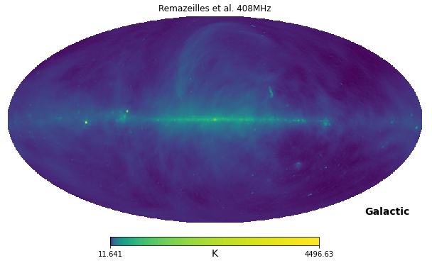
Figure 3 . The all-sky 408Mhz map from AD1, used to calculate \(T_{408}\).
Efficiencies
Aperture
Following RD2, the aperture efficiency \(\eta_A\) is given by:
where:
and:
\(\eta_{dish}\) accounts for the efficiencies attributable to the dish optics
\(\eta_{block}\) accounts for physical aperture blockage
\(\eta_{transp}\) accounts for losses by transmission through the reflector surface
\(\eta_{surface}\) accounts for all losses due to incoherent propagation through the optics, including panel roughness, systematic deformation and mis-alignment;
\(\eta_{rad.r}\) accounts for the Ohmic dielectric and scattering losses in the reflector system only
\(\eta_{feed}\) accounts for the efficiencies attributable to the feeds
\(\eta_{rad.f}\) accounts for feed mismatches and losses
\(\eta_{ill}\) is the efficiency due to the actual illumination pattern
Currently, the SC follows RD1 and calculates an overall \(\eta_{dish}\) from estimates of \(\eta_{ill}\), \(\eta_{surface}\) and \(\eta_{diffraction}\) (?).
Array
The system efficiency \(\eta_s\) is the result of multiplying together the following factors:
eta_bandpass This factor describes the loss of efficiency due to the departure of the bandpass from an ideal, rectangular shape. At present the value is set to 1.0.
eta_coherence This factor desribes the loss of efficiency due to coherence loss on a baseline.
\[\eta_{coherence} = \exp-\frac{<\phi_{\epsilon}^2 (t)>}{2} = \exp-2\pi ^2 \nu_0^2 <\tau_\epsilon ^2(t)>\]We take the coherence loss at 1s integration time, which is white phase-noise dominated. The total phase delay is due to the sum in quadrature of the phase delay of the clock and signal path on both receptors:
\[<\tau_\epsilon ^2> = <\tau_{clk,i}^2> + <\tau_{clk,j}^2> + <\tau_{dsh,i}^2> + <\tau_{dsh,j}^2>\]The signal path depends on the environment (atmosphere, gusty wind) and the calibration quality, which is quite complicated to estimate in practice. For now we adopt a value of \(\eta_{coherence} = 0.98\) at \(\nu_0 =15.4GHz\) as coherence loss for the worst case, and scale it to the frequency of observation using the given formula.
eta_correlation This factor describes the loss of efficiency due to imperfection in the correlation algorithm, e.g. truncation error. Analysis described in “SKA CSP SKA1 MID array Correlator and Central beamformer sub element Signal Processing Matlab Model” (311-000000-007) shows that the CSP correlation efficiency is almost 100% in the case of zero RFI, and better than 98% in the case of strong RFI (defined as <10% RFI in the outside visibility ?query, what does this mean).
Currently the efficiency value is set to 0.98.
eta_digitisation This factor describes the loss of efficiency due to quantization during signal digitisation. The process is independent of the telescope and environment, and depends only on the ‘effective number of bits’ (ENOB) of the system, which depends in turn on digitiser quality and clock jitter, and on band flatness.
The values used for each band are as follows:
Band
ENOB
Band Flatness (dB)
\(\eta\)
Band 1
8
6.5
0.999
Band 2
8
6.5
0.999
Band 3
6
6.5
0.998
Band 4
4
6.5
0.98
Band 5a
3
4 (in any 2.5GHz BW)
0.955
Band 5b
3
4 (in any 2.5GHz BW)
0.955
eta_point This factor describes the loss of efficiency due to dish pointing errors. Here we currently use an approximate formula:
\[\eta_{point} \sim \frac{1}{1 + 8 ln2 \frac{\sigma_{\theta}^2}{FWHM^2}}\]where FWHM is the beam full-width at half maximum power for the dish, given by the approximate formula \(FWHM \sim 66 \lambda / D\) (degrees), and \(\sigma_\theta\) is the RMS pointing error.
Design Independent
This section lists efiiciency factors that are independent of the telescope design.
eta_rfi This factor describes the loss of efficiency due to parts of the spectrum that are lost due to strong RFI noise corrupting the astronomical signal. Currently set to 1.
eta_data_loss This describes the loss of observing time due to the need for calibration, time spent moving to source, etc.
It is currently not used in the calculator, so implicitly set to 1.
Sensitivity Degradation due to RFI
The effect of RFI is not currently included in the system efficiency budget.