Introduction

The following is documentation for users of the SKA-Low system. This documentation is intended to help users understand the system and how to interact with it.

Acquire Access

There are two (and a half) main clusters that you can access:

SKA-Low: This is the main cluster where you can use the actual stations (currently s8-1, s8-6, s9-2 and s10-3). This is actually split into two clusters:
- North MCCS: The cluster located on the MRO site which controls the SPS hardware which is primarily MCCS. This cluster is used to launch station observations with the low level MCCS software and to turn stations on.
- South Pawsey: The cluster located at Pawsey which controls the data processing and other software components (TMC, SPS and CBF). This cluster is used to launch observations with the high level TMC software.
ITF: The integration test facility where you can use test software with generated signals

There are two ways to access the clusters:

JupyterHub: This is a web-based interface that allows you to run notebooks on the cluster. This is the easiest way to get started.
k9s/kubectl: This is a terminal-based interface that allows you to look at individual pod’s logs and kill them if necessary. This is more advanced and is useful for debugging.

ITF Cluster

To access the ITF cluster, submit a system team ticket to request VPN access. You will need to install the cisco VPN client on your machine and connect to the SKAO VPN before you can access the cluster.

You should then be able to access the ITF JupyterHub interface at https://k8s.lowitf.internal.skao.int/jupyterhub/hub. You will have to login with your SKA and GitLab credentials then click launch server. When you launch the server for the first time, several things will be installed which may cause the launch to time out. If this happens, try again a few times until you can see the JupyterLab interface.

If you plan to use the Tango devices, first make sure that no one else is using the ITF cluster, then reserve time using the calendar.

SKA-Low MCCS Cluster

To access the SKA-Low MCCS cluster, send a message (or email lucio.tirone@csiro.au) to Lucio Tirone to request VPN access (by adding you to the correct security group).

Make sure you are connected to the SKAO VPN and then you can access the SKA-Low JupyterHub interface at https://k8s.mccs.low.internal.skao.int/jupyterhub/hub. You will once again have to login with your credentials and have to try a few times until you can see the JupyterLab interface.

If you plan to use the Tango devices, first make sure that no one else is using the station you plan to use by checking the calendar. To reserve a station follow the instruction at the bottom of the calendar page.

k9s/kubectl Interface

k9s is a terminal-based interface that allows you to look at individual pod’s logs and kill them if necessary. Because this has the ability to kill pods, you will only be granted access if you are a more advanced user (such as part of the Vulcan team). To install k9s, follow the instructions on the k9s website.

To access the k9s interface, you will need to be connected to the SKAO VPN and be granted access through InfraHQ. After you have downloaded and installed infra, follow the SKA instructions to login. If you have the correct permissions, the command infra list will show you the available clusters, which should include au-aa-mccs-cloud01-k8s for SKA-Low MCCS cluster and au-itf-k8s-master01-k8s for the ITF cluster.

Useful Link Summary

Many of the following links are mentioned and explained in other sections, but for your convenience, here is a summary of useful links:

SKA-Low North MCCS
- JupyterHub
- Calendar (same for SKA-Low)
- Grafana (deprecated as all North Grafana dashboards are also in the South Grafana)
- Taranta
- Kibana (same for SKA-Low)
SKA-Low South Pawsey
ITF
Repositories
- SKA-Low Tests
- SKA-Low Deploy
Documentation

High Level Overview

Telescope Components

An interferometer takes signals from multiple receivers and compares them over time. By applying a specific mathematical transformation to these comparisons, an image can be formed.

In SKA Low, the receivers are stations, which consist of a set of antennas whose signals are added together as a phased array to form station beams. The comparison between station beams is performed by the Correlator and BeamFormer, or CBF, which is a part of the Central Signal Processor, or CSP. The number crunching to take the outputs from CSP and produce images and other scientific products is performed by the Science Data Processor, or SDP, and this whole process is orchestrated by Telescope Monitoring and Control software, or TMC.

Note

Why is it called the correlator and beamformer if beams are already formed in MCCS?

Beamforming can happen at multiple levels - antenna signals are summed by the Tile Processing Modules (TPMs) to create station beams, and then those station beams may be summed by CBF to form extremely sensitive tied-array beams, which aren’t useful for imaging but are great for analysing time-domain phenomena like pulsars.

So, the software subsystems in play are:

MCCS, the Monitoring, Calibration and Control Subsystem - this is responsible for controlling the Low station hardware that captures, digitises and sums antenna signals. MCCS is also responsible for calibrating stations, and capturing engineering sample data from stations.
CSP, the Central Signal Processor - receives station beams from site, and does further cross-station processing, either correlating or further beamforming.
SDP, the Science Data Processor - takes products from CSP for further processing, e.g. creating images. Currently, SDP simply receives and stores visibilities from CSP.
TMC, Telescope Management and Control - the high-level control system which coordinates all the other subsystems in order to perform a scan.

MCCS, CSP, and SDP are functional subsystems which each implement a portion of the telescope signal chain. Each of these has a controller and its own representation of a subarray, implemented as Tango devices. The controller is responsible for turning things on and off, and for allocating resources within its subsystem to subarrays.

These functional subsystems are controlled by TMC, which also has its own representation of a subarray.

MCCS

The Monitoring, Calibration and Control Subsystem control system is loosely hierarchical. The primary interface to a Low station is an MccsStation Tango device. This device should represent the aggregate state of all station hardware, and provide commands to operate a station as an atomic unit. Unfortunately this abstraction is not watertight, so it’s often necessary to interact with devices beneath MccsStation in the hierarchy.

The next tier of devices are SpsStation, and FieldStation. These correspond to the two main functional areas of the hardware under MCCS control - PaSD and SPS.

(MCCS should also theoretically monitor and control the synchronisation and timing system (SAT) and infrastructure like Power Distribution Units (PDUs) and chillers, but this functionality is immature as of September 2024.)

MCCS Tango devices for high-level control
Tango device name	comment
MccsController	allocates resources to subarrays, turns the array on and off
MccsStation	represents a station, both the field node and signal processing system
MccsStationBeam	a station may eventually have up to 48 beams, each of which is configured for a specific subarray beam
MccsSubarray	MCCS’ internal representation of a subarray
MccsSubarrayBeam	a beam for a specific target and frequency that may be instantiated in multiple stations

There are three devices dedicated to calibration:

MCCS Tango devices for calibration
Tango device name	comment
StationCalibrationSolverDevice	a service device for performing calibration calculations
MccsStationCalibrator	orchestrates calibration: acquiring sample data, calculating and applying calibration solutions
MccsCalibrationStore	stores calibrations solutions?

PaSD

FieldStation represents the Power and Signal Distribution (PaSD) system, which consists of the hardware that sits outside in the weather alongside the antennas - 24 smartboxes and one field node distribution hub (FNDH). The science inputs to this system are the sky, and the outputs are analogue optical signals on fibres, one per antenna.

PaSD hardware and Tango devices are initialised by the FieldNodeOn.ipynb: operational notebook.

PaSD Tango devices are developed in the https://gitlab.com/ska-telescope/mccs/ska-low-mccs-pasd repository by the Wombat and MCCS teams.

MCCS Tango devices for hardware components
Tango device name	hardware component	comment
FieldStation		An abstract device representing a field node
MccsFNDH	field node distribution hub	sits on the edge of the mesh, and powers and controls smartboxes
MccsPasdBus	ethernet-modbus gateway	The central point of communication with all PaSD hardware. This is the only PaSD Tango device that directly communicates with hardware.
MccsSmartbox	smartbox	contains up to 12 FEMs (front-end modules) which convert an electrical signals from antennas into optical signals on fibre

SPS

SpsStation represents the Signal Srocessing System (SPS) for a station. This is high-performance dedicated computing hardware (tile processing modules or TPMs) that lives in climate controlled, EM-shielded structures: either remote processing facilities in the case of stations on the spiral arms, or the central processing facility in the case of stations in the core. The TPMs take analogue optical input from the PaSD, digitise them, add them together and send the resulting station beams to CSP.

The SPS hardware and Tango devices are initialised by the Initialise.ipynb: operational notebook.

SPS Tango devices are developed in the https://gitlab.com/ska-telescope/mccs/ska-low-mccs-spshw repository by the MCCS team. Within MCCS is a specialist team who develop the signal processing firmware that runs on the TPMs.

MCCS Tango devices for hardware components
Tango device name	hardware component	comment
SpsStation		An aggregate device representing the set of 2 subracks and 8 TPMs in for a station.
MccsTile	TPM	Tile processing module - digitises and beamforms antenna signals
MccsSubrack	subrack	Each subrack distributes power and LMC network to 8 TPMs
MccsDaqReceiver		A software device which receives data samples from TPMs for engineering and calibration purposes

CSP

The Central Signal Processor is responsible for correlating or beamforming the signals from stations and performing further processing for pulsars. Unlike MCCS, there are no Tango devices at the top level - high-level control is provided by the CSP-LMC component.

The CBF is implemented on special-purpose Commercial Off the Shelf (COTS) hardware - FPGAs and programmable P4 switches, of which there are six and one respectively in Low AA.

PSS and PST are implemented in software and run on COTS server hardware.

CSP-LMC

CSP-LMC Tango devices for high-level control
Tango device name	comment
CspController	allocates resources to subarrays, turns the array on and off
CspSubarray	CSP’s internal representation of a subarray

CBF

CBF Tango devices for control of the correlator and beamformer
Tango device name	hardware component	comment
CbfAllocator		allocates CBF hardware components (i.e. FPGAs) for particular observations
CbfConnector	P4 switch	controls the programmable P4 switch by dynamically configuring routing of station beams to FPGAs
CbfProcessor	Alveo FPGA	programs and commands the FPGAs on which the actual correlation and beamforming take place

PSS and PST

The PulSar Search (PSS) and PulSar Timing (PST) systems are software components to process the high time resolution pulsar data.

TODO - these are so far undeployed in the Low ITF or in Low AA.

SDP

Science Data Processor has no specialised hardware, and uses less Tango than other areas of the signal chain. SDP relies Kubernetes as a part of its internal operation, using Helm to create on-demand deployments of Pods for receiving data and running scripts for observations. Much of this is unexposed to the Tango world.

SDP manages its state in an internal etcd database.

It still provides Tango devices for its high-level control interface:

SDP Tango devices for high-level control
Tango device name	comment
SdpController	allocates resources to subarrays, turns the array on and off
SdpSubarray	SDP’s internal representation of a subarray

TMC

Telescope Monitoring and Control provides the highest-level Tango devices for controlling the telescope. The main public interfaces are the TmcCentralNode and TmcSubarrayNode. Internally, TMC also has Tango devices coupled to each of the subsystems’ subarray devices and to their controllers.

TMC Tango devices for top-level control
Tango device name	comment
CentralNode	allocates resources to subarrays, turns the array on and off
SubarrayNode	SDP’s internal representation of a subarray
CspMasterLeafNode	TMC’s proxy to CspController
CspSubarrayLeafNode	TMC’s proxy to a CspSubarray device
MccsMasterLeafNode	TMC’s proxy to MccsController
MccsSubarrayLeafNode	TMC’s proxy to an MccsSubarray device
SdpMasterLeafNode	TMC’s proxy to SdpController
SdpSubarrayLeafNode	TMC’s proxy to an SdpSubarray device

ITF Signal Generators

The ITF has a set of sky signal generators which are used to simulate the signals from antennas. How to use the signal generators is described in LOW-ITF Usage Procedure. There is also two Taranta dashboards that can monitor and control the switches and the sky signal generators. If either of these dashboards are not available, notify the Vulcan team so they can redeploy them from the ITF repository.

Kubernetes

Kubernetes is a container management system. Functionality is divided into groups of containers (“Pods”) which can be deployed amongst many servers (“Nodes”) to share the load. The total set of nodes and pods form a “cluster”. See https://kubernetes.io for more information.

The kubernetes system is used by SKAO so that we can automatically role out new software versions of the different components and roll back these versions if there are any issues with new releases. It also makes the cluster more fault tolerant as if one part of the telescope fails, then that pod can be killed and a new one will automatically be generated to take its place.

Clusters

Currently, the SKAO has three Clusters:

Cluster	Infra Context	Location
Low ITF	infra:au-itf-k8s-master01-k8s	Geraldton ITF
SKA-Low North (MCCS)	infra:au-aa-mccs-cloud01-k8s	Low AA Site tcpf
SKA-Low South (Pawsey)	infra:au-aa-k8s-master01-k8s	Pawsey Centre

See the Acquire Access section if you haven’t already been given access.

Pods

A pod is the smallest unit in the Kubernetes ecosystem. Kubernetes uses the description of the pod to assign it resources such as storage and ram, which container it shall use and other start up commands. These pods are ephemeral which allows automatic restarts in the case of failure.

Pods can be grouped into namespaces for easier management. The logs for a given pod can be also be viewed using Kibana, k9s or kubectl (see Kibana, k9s and kubectl sections).

For SKAO, you can think of each pod contains a docker container that contains a tango device which interacts with hardware or other tango devices.

Tango

Tango is a control system framework for physical hardware (as well as software abstractions). SKAO uses the python binding PyTango to create devices representing elements of the Telescope (such as TPMS and subarrays) as well as test equipment (e.g. an Arbritrary Waveform Generator (AWG) or a Noise Source). After definition and deployment to a cluster, these devices can be used from scripts or Jupyter Notebooks remotely.

Tango Device Servers and Proxies

The Tango devices are managed by a Tango Device Server which we can get DeviceProxy instances from. This device proxy is a class that can communicate with the tango device that is being run in a different kubernetes pod which in turn talks to hardware.

For example, on the ITF we can get a device proxy for an Arbitrary Waveform Generator (AWG) like this:

from tango import DeviceProxy
trl = "tango-databaseds.test-environment:10000/low-itf/awg/1"
awg = DeviceProxy(trl)

We used the Tango Resource Locator (TRL) for the AWG to get a device proxy that we interact with in Jupyter Notebooks.

The TRL shows the tango database name and port, along with the device name. In the case of SKAO, the tango database is in kubernetes which is partitioned into namespaces, so the namespace qualifier is used. We do this because the MCCS and other devices are split across two clusters so they require different TANGO_HOST s. To make this easier to handle, Vulcan has made wrapper scripts for grabbing devices with the shorter TRLs (which you can see at the top of the Taranta when you click on a device):

from aiv_utils.low_utils import get_device, get_mccs_device
station = get_mccs_device("low-mccs/station/s8-1")
tmc_subarray = get_device("low-tmc/subarray/01")

To see a list of tango device servers (pods) residing in a given namespace one can use kubectl, k9s or Taranta (see Useful Link Summary). You can also directly get the list from the tango database using the following code:

from tango import Database
db = Database()
list(db.get_device_exported("*"))

Or for MCCS devices:

from aiv_utils.low_utils import get_mccs_tangodb
db = get_mccs_tangodb()
list(db.get_device_exported("*"))

The Vulcan group have made several helper functions to get some of the device proxies for you. For example, to get the Signal Processing System (SPS) device proxies you can use:

from aiv_utils.low_utils import get_sps_devices
STATION_NAME = "itf1"
sps_station, subracks, tpms, (daq, bandpass_daq) = get_sps_devices(STATION_NAME)

or the following so handle almost everything else:

from aiv_utils.low_utils import (
    get_cbf_devices,
    get_csp_devices,
    get_mccs_devices,
    get_pasd_devices,
    get_sdp_devices,
    get_stations,
    get_tmc_devices,
)
STATION_NAME = "itf1"

stations = get_stations()
field_station, pasdbus, fndh, smartboxes = get_pasd_devices(STATION_NAME)
(
   mccs_controller,
   stations,
   mccs_subarrays,
   mccs_subarray_beams,
   station_beams,
) = get_mccs_devices()
csp_controller, csp_subarrays = get_csp_devices()
(
   cbf_controller,
   allocator,
   connector,
   processors,
   delaypoly,
   cnics,
   cbf_subarrays,
) = get_cbf_devices()
sdp_controller, queue_connectors, sdp_subarrays = get_sdp_devices()
(
   central_node,
   csp_master_leafnode,
   csp_subarray_leafnodes,
   mccs_master_leafnode,
   mccs_subarray_leafnodes,
   sdp_master_leafnode,
   sdp_subarray_leafnodes,
   tmc_subarray_nodes,
) = get_tmc_devices()

These helper functions are documented in the API section.

Each tango device consists of sets of Attributes and Commands that can be read and executed respectively.

Attributes

Attributes are typed variables representing features of the device (e.g. frequency, temperature). To see a list of attributes for a given device type: device.get_attribute_list()

Attribute Operations
Operation	Example Code	Explanation
List available device attributes	`awg.get_attribute_list()`	This will work for all devices
Read Attribute	`awg.frequency`	Use dot notation: device.attribute
Write Attribute	`awg.frequency = 250e6`	Assignment of new value
Change AdminMode	`awg.adminMode = 0`	Change the AdminMode to online (see next section for explanation)

Admin Mode

Each Tango device has an AdminMode attribute of which there are three states that we use:

ONLINE (AdminMode=0): Indicates that the component/subarray can be used for scientific observations and communicating with hardware
OFFLINE (AdminMode=1): An AdminMode of OFFLINE means that the software will not do any monitoring and control. We set AdminMode to OFFLINE to turn off communication with the hardware. (note this will be replaced once ADR-114 is implemented)
ENGINEERING (AdminMode=2): Indicates that the component/subarray is reserved to be used for engineering purposes (this includes a wide range of activities, such as commissioning, testing, maintenance, etc).

There are some Tango devices, such as the MCCS SPSHW station device, which require being in engineering mode to run certain commands, such as turning on the test signal generator. If you require a device to be in Offline or Engineering Admin Mode, it is best to put a booking in the calendar to let people know what station/device, why and for how long. It may also be useful to send a message on the relevant Slack channels (#team-low-aa1) for any last-minute or important changes. This communication will prevent someone from reverting your device to Admin Mode Online.

If you wish to turn the station/device back to Admin Mode Online, first check why the device is in Engineering/Offline mode. This can be done by checking if there are current or recent bookings on the calendar. This calendar webpage does not update automatically so it is best to refresh the page every time you want to check it. If there was a recent booking, it is best to send the person a message to confirm they have finished using the device. Once you have confirmed there is no reason the device needs to be in a different Admin Mode, you can then return it to Admin Mode Online using the Taranta web interface (see the Taranta section for details) or JupyterHub with code like the following. There are helper functions to make using Tango devices easier, explained in the Tango Device Servers and Proxies section.

from ska_control_model import AdminMode
from aiv_utils.low_utils import get_sps_devices

STATION_NAME = "s8-1"
sps_station, subracks, tpms, (daq, bandpass_daq) = get_sps_devices(STATION_NAME)
sps_station.adminMode = AdminMode.ONLINE

Commands

Commands are operations a device can perform.

Commands
Operation	Example Code	Explanation
List available commands	`awg.get_command_list()`	This will work for all devices
Execute a command	`awg.Play()`
Execute a command with arguments	`car.Turn(90)`

Depending on the Tango Device, commands can be synchronous (blocking), where the user must wait for the command to finish or asynchronous (long running commands) which return immediately. The execution status of a long running command can be checked by issuing: device.longrunningcommandstatus

Tango Events

Tango devices emit events when attributes are changes or commands are run. Clients can subscribe to these events and add custom event handlers.

For example, a subscription looks like:

subscription_id = deviceproxy.subscribe_event(attribute, tango.EventType.CHANGE_EVENT, event_handler, [])

Where event_handler is any python function

To unsubscribe you can then run:

deviceproxy.unsubscribe_event(subscription_id)

Using and Monitoring the System

JupyterHub

JupyterHub is a web-based interface that allows you to run notebooks and terminal commands on the cluster. In the following sections we will describe the directories available to you and the basics of how to use JupyterHub.

Directories

When you first open JupyterHub, you will see a list of directories in your home directory on the cluster (/home/jovyan/). Some are mounted volumes that are shared with all users, such as daq-data, eep-data, sdp-data, cnic-data and shared.

The shared directory is where you can put data that you want to share with other users. It is recommended that you make a directory with your username in the shared directory and put your data there. The daq-data directory is where the data from the daq is stored. The eep-data directory is where the EEP simulated data files are stored. The sdp-data directory is where the data from SDP is stored which includes TMC observations. The cnic-data directory is where the Customisable Network Interface Card (CNIC) simulated data files are stored.

All other directories currently in /home/jovyan/ or that you create are only accessible by you. These means that any changes you make to the operational notebooks or the aiv_utils package will not affect other users. If you have made a change that will benefit others, see the Contributing to the ska-low repository section for an explanation of how to contribute.

The Launcher

If you press the blue + button in the top left of the JupyterHub interface, you will see a list of options for creating new files or terminal. If you open a terminal, you can run shell commands as normal which is useful for running git commands to ensure you are using the most up-to-date version of the operational notebooks and aiv_utils package. You can also open a new notebook or python console from the launcher. Make sure you select the Python 3 (ipykernal) option so that you have access to the aiv_utils package.

Jupyter Notebooks

Jupyter Notebooks are a way to run python code interactively. They are made up of cells which can be run individually. The default command to run a cell is Shift + Enter which you can press for each cell to run the whole notebook or click ⏩ in the toolbar to restart the kernel and run all cells.

If you want to keep the output of the cells, the easiest way is to copy the notebook and give it a new filename before rerunning it. If you want to clear the outputs (before git committing changes for example) you can click “Edit” then “Clear All Outputs”.

Grafana

Grafana is an open-source visualisation platform for the creation of near realtime charts and displays. The primary source of data displayed in the SKAO Grafana is the Engineering Data Archive (EDA), for more information see the Grafana Dashboards and the EDA database section To view the dashboards you must be connected to the VPN.

Low ITF Dashboard Homepage provides links to all dashboards.
SKA-Low Dashboard Homepage provides links to all dashboards.

Common error messages displayed on the Subarrary dashboard

The Subarray dashboard contains two panels that can provide additional debugging information when observations fail, “Command Results” and “Failed LRC commands, most recent first”. You can click a failed command and then click the tooltip to copy the full error message. The first of these shows a timeline view aligned with the above ObsState panel. Hovering over the commands listed in the panel will provide additional information if they have failed. The “Failed LRC commands, most recent first” panel shows all of the commands that have failed in the time period in more detail. Below is a list of common error messages, an explanation of why they may have occurred, and any steps that can be done to resolve the issue. This should be regularly updated. Contact @teamvulcan on Slack if this needs updating.

Error message

Component

Explanation

Steps to fix

Configure FAILED {“low-mccs/subarraybeam/01-01/Configure”: {“action”: “low-mccs/subarraybeam/01-01/Configure”,”result_code”: “FAILED”,”result_info”: {“low-mccs/beam/s10-3-01/Configure”:{“action”: “low-mccs/beam/s10-3-01/Configure”, “result_code”: “FAILED”,”result_info”: “Unhandled exception during execution: Component is not powered ON”}}}}

MCCS

For an observation to succeed, all of the stations assigned to that subarray must be online. Stations consist of a FieldStation (to get signal from the antennas) and an SpsStation (to process the signal). Both of these must be ONLINE for the station to be considered ONLINE and able to observe.

Turn on the field node (run FieldNodeOn.ipynb) if FieldStation is OFF or UNKNOWN.

Initialise the station if SpsStation is in STANDBY.

AssignResources ABORTED CM method connect_to_pst not executed due to an abort request in progress. LRC command assignresources on low-cbf/subarray/04 not executed due to an abort request in progress.

CBF

This is SKB-1126. More information can be found in the ticket.

Contact @teamvulcan and ask for the devices to be restarted.

Configure FAILED cbf-subarray-01: Unhandled exception during execution: Action configure_completed is not allowed in obs state ABORTING.

CBF

Certain commands can only succeed in certain observation states. This is a minor CBF bug where configure_completed is called even while CBF is in aborting. This does not affect observations in any way and should be ignored for now.

Nothing to fix, does not affect observations.

Kibana

Kibana is a web interface primarily for searching and visualizing logs. It is useful for investigating the logs of the various Tango pods when you encounter an issue. Currently, only the ITF cluster has Kibana enabled.

To access Kibana, you must be connected to the VPN, then navigate to the following links: - ITF Kibana - SKA-Low Kibana

The stream will be overwhelming at first because it will display all logs from the cluster (not just pod logs). You can add several filters to the be more specific about the logs you want to see.

You often will want to see the logs for pod of the Tango DeviceProxy that gave you an error. You can use the device name as a filter to only see logs from that pod. You can get the device name with the .dev_name() command:

from aiv_utils.low_utils import get_sps_devices
STATION_NAME = "itf1"
%env TANGO_HOST=tango-databaseds.sut-mccs:10000
station, subracks, tpms, (daq, _) = get_sps_devices(STATION_NAME)

station.dev_name()

which outputs

'low-mccs/spsstation/itf1'

You can add a filter to Kibana to only see logs from this pod by adding the following filter in the filter bar: ska_tags_field.tango-device : low-mccs/spsstation/itf1

You may also need to change the time range to see logs from the time you encountered the error. You can do this by clicking the calendar icon in the top right and selecting the time range you are interested in.

You can use more than one filter at a time by separating them with an “ and “ in the filter bar. The following filters may be useful:

ska_severity : "ERROR" Only look for error messages (filter our warnings and info messages)
ska.application : kubernetes Only look for logs from the kubernetes pods (ignore cluster logs)
kubernetes.namespace : sut-mccs Only look for pods of a certain namespace if you’re only interested in MCCS devices for example
message : *Failed to connect* Find logs that contain the phrase “Failed to connect” or any other phrase you are interested in
kubernetes.pod.name : spsstations-spsstation-itf1-0 Find logs from a specific pod
ska_tags_field.tango-device : low-mccs/spsstation/itf1 As mentioned above, find logs for a Tango device’s pod

Taranta

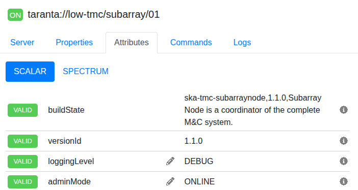
Taranata is an interactive web page (see Useful Link Summary for each cluster’s link) for monitoring and controlling Tango devices. The Tango devices are organised into sub-system then device type. You can use Taranata to check the attributes of Tango devices without having to know their exact names.

If you log in (ask Vulcan for log in credentials) then you can change some of the attributes (such as AdminMode) and send commands (such as On and Off). After logging in, you can change attributes by clicking on the pencil icon and choosing the desired value.

k9s

If you have the correct permissions (see k9s/kubectl Interface), you can use the graphical tool k9s to investigate and manage a cluster. Make sure you install k9s (and for full functionality also install kubectl) Then once you have logged in with infra login and connected to the VPN you should be able to use k9s to connect to the clusters.

Once in the k9s interface, make sure you are in the correct cluster (Clusters) which can be chosen using the :context command. You may then also have to press 0 to see all the namespaces in the cluster. You may then want to use / to filter the pod names to find what you are interested in. For example I could type /daq then click enter to see all the daq pods or /s8-6 to see all the pods for the s8-6 station.

Once you have found the pod you are interested in, you can click l to see the logs, d to describe the pod or Ctrl + k to kill the pod (don’t do this lightly!). Investigating the pods in this way can help you to understand what is happening in the cluster and debug any issues.

kubectl

If you want a more advanced command line tool, you can use kubectl to view and modify the cluster. Some common commands are shown below.

kubectl commands
Action	Example Command Line
List contexts (clusters)	`kubectl config get-contexts`
Use a context (cluster)	`kubectl config use-context infra:au-itf-k8s-master01-k8s`
List namespaces in a cluster	`kubectl get namespaces`
List all pods in namespace	`kubectl -n sut get pods`
Show logs of a given pod in a namespace	`kubectl -n sut logs centralnode-01-0`

Using SKA-Low Tests Notebooks and Tools

When the JupyterHub server is launched, the SKA-Low Tests repository is cloned and fetched in the directory /home/jovyan/ska-low. The most important two directories in this repository are:

ska-low/notebooks/operations: This directory contains the notebooks that are used for common operations such as initialisation of stations and acquiring data.
ska-low/src/aiv_utils: This directory contains the helper functions that are used in a lot of the notebooks.

Operation Notebooks

The operation notebooks cover common station operations such as initialisation, data acquisition, and calibration. Each notebook is internally documented and should explain each step they take. All of these notebooks are intended to run on the North MCCS cluster with the exception of the TMCObservation.ipynb notebook which should be run on the South Pawsey cluster. Because the ITF is not two distinct clusters like SKA-Low, all the operation notebooks can be run on the ITF. We will now go through the purpose of each operation notebook in the ska-low/notebooks/operations to make it clear how they should work together.

TMCObservation.ipynb: This notebook uses the high level TMC software to observe with one or more stations. This is the only operation notebook that needs to be run on the South Pawsey cluster (or the ITF). The output data is stored in the /home/jovyan/sdp-data directory. For imaging observations, the data will be visibilities in the measurement set format; for tied-array beam observations, they will be voltage data in dada format. For more detail on how to use this notebook and how to calibrate before the observation, see the TMC Observation Notebook and Applying Calibration in TMCObservation.ipynb sections.

FieldNodeOn.ipynb: This notebook will attempt to get a field node into the state where the FNDH and all smartboxes are initialised and all FEM ports on. This notebook should be run after any maintenance that might required the field node to be turned off or if output data is not as expected (none or too small to look like a bandpass).

Initialise.ipynb: This notebook will bring the station up to the point where TPMs have started acquisition. If the station has just been powered on, this notebook will have to be run after FieldNodeOn.ipynb. If all the TPMs are in a synchronised programming state (can be confirmed on the station overview dashboard), then this notebook does not need to be run. If the station is behaving unexpectedly (such as data files not being written) then reinitialising the station is a good first debug step.

Equalise.ipynb: This notebook will attempt to equalise the station by adjusting the preadu levels so that each antenna emits similar amounts of power. The Initialise.ipynb now applies a default preadu levels from the TelModel, so this notebook is only necessary if the bandpasses are starting to noticeably drift.

ManageStationCalibrationLoop.ipynb: This notebook is used for starting and stopping the station calibrator device. The calibration loop constantly acquires correlation data and calculates calibration solutions from it. If you want to run a daq based observation, you will need to stop the calibrator before starting your observation. TMC-based observations are unaffected by the station calibrator loop running.

FrequencySweep.ipynb and FrequencySweepMultiple.ipynb: These notebooks acquire correlator data from one station (FrequencySweep.ipynb), or one or more station (FrequencySweepMultiple.ipynb). FrequencySweep.ipynb is used for a single station and creates some extra plots to help with debugging, internally it runs FrequencySweepMultiple.ipynb where the list of stations contains a single station name. FrequencySweepMultiple.ipynb is used for multiple stations which start simultaneously. Such data are used to calculate calibration solutions.

06.Calibration.ipynb *: This notebooks is not technically an operation notebook, but it is used to generate calibration solutions for the stations. The notebook can be found in the ska-low/notebooks/SFT/06.Calibration directory and is further explained in the Calibration section.

AcquireBeamformed.ipynb: This notebook acquires beamformed data for one or multiple stations. For details on how to acquire beamformed data with calibration applied, see the Applying Calibration in AcquireBeamformed.ipynb section.

AcquireMultiBeam.ipynb: This notebook acquires multi-beam beamformed data for one station using an json file specifying pointings within the observation. The primary use of it is to be called using papermill by the multi-beam SFTs.

AcquireRaw.ipynb: This notebook acquires a burst of raw voltage data for a station.

AcquireChannelised.ipynb: This notebook acquires a burst of channelised data for a station.

AcquireContinuousChannelised.ipynb: This notebook acquires a burst of channelised data for a station.

TMC Observation Notebook

The TMCObservation.ipynb notebook uses higher level software than other operational notebooks and is what will be use most often for science observations. The following will describe how to decide on the parameters for the observation and how to run the notebook.

The STATION_NAMES variable is a list of stations you want to use, e.g. STATION_NAMES = ['s8-6', 's9-2']. You should check that the stations are available and you have booked them on the calendar and they are in a good state by checking the station overview dashboard.

To choose what type of observation the scan will be, set OBSERVING_MODE to either:

VIS: Which will output imaging visibilities and is explained in the SDP Visibility Observations section.
PST: Which will output high time resolution voltages and is explained in the PST Voltage Observations section.

The calibrations for each station can be set using the CALIBRATION parameter. It should be set as a list of strings of either "FROM_STORE", "UNITY" or "ZERO" for each station. Leaving this blank will default to using the golden calibration solutions from the store. For more information on the calibration, see the Applying Calibration in TMCObservation.ipynb section.

The final paramater to set is OBSERVATIONS which is a list of dictionaries that define the observations. Each dictionary should have the following:

"Observation name": A string that describes the observation. There is no parsing/validation on the string but it is good practice to use the official source name as it will be recorded in the metadata.
"RA (deg)": The Right Ascension of the source in degrees.
"Declination (deg)": The Declination of the source in degrees.
"Duration (min)": The duration of the observation in minutes. This should be a minimum of 0.5 minutes (30 seconds) for PST observations.
"Start frequency channel ID": The lowest coarse frequency channel ID for the observation. This must be an even number and can be multiplied by 0.78125 to get the frequency in MHz (e.g. channel 64 is 50 MHz).
"Bandwidth channels": The number of coarse frequency channels to use for the observation. This must be a multiple of 8 and is currently recommended to be 24 or less for VIS observations so only a single SDP receiver is used which gives more consistent results (see SKB-701 and SKB-695). It is recommended to set it to 8 for PST observations so the filesystem can keep up with disk writes, and packets are not dropped.

You can set multiple observations by listing multiple dictionaries in the OBSERVATIONS list. The notebook will ReleaseResources() and AssignResources() between each observation (until SKB-701 is resolved). For example, two observations could look like this:

OBSERVATIONS = [
    {
        "Observation name": "CasA",
        "RA (deg)": 350.85,
        "Declination (deg)": 58.81,
        "Duration (min)": 5,
        "Start frequency channel ID": 64,
        "Bandwidth channels": 8,
    },
    {
        "Observation name": "CygnusA",
        "RA (deg)": 299.868,
        "Declination (deg)": 40.7339,
        "Duration (min)": 5,
        "Start frequency channel ID": 64,
        "Bandwidth channels": 8,
    },
]

Once the parameters are set you can either use Shift + Enter for each cell to run the whole notebook or click ⏩ in the toolbar to restart the kernel and run all cells. You can then use the subarrays dashboard to monitor the progress of the subsystems from EMPTY to IDLE to READY to SCANNING. Once the system has got to scanning it is normally smooth sailing but you can check the CBF connector dashboard to confirm data is flowing (mostly only used by Vulcan for debugging) or the SDP signal display dashboard to monitor the real time visibility data.

The data will be stored in the /home/jovyan/sdp-data directory and the exact location will be printed in the notebook. See the following sections for descriptions of the observation mode dependent data formats.

PST Voltage Observations

The “PST” observations are high time resolution voltage data which can be used for pulsar observations. The data sizes are very large so please be careful about observation length until the PST real time folding is implemented (currently waiting on PST hardware before the software can be integrated). The data will be output to the /home/jovyan/sdp-data/<eb_id>/pst-low/1 directory where <eb_id> is the execution block ID which can be found in the notebook outputs or should be the most recent directory in /home/jovyan/sdp-data/ if you just observed. The files in this directory include:

scan_configuration.json: The configuration given to the subarray nodes for the observation.
ska-data-product.yaml: A summary of the metadata of the observation. This is calculated after the observation finishes so will accurately describe the files, for example if the observation did not record data then t_exptime will be 0.
data: A directory of the raw voltage files in dada format.
weights: A directory of the weights files in dada format. These are used to adjust the data files to account for the different gains used throughout the observation.
stats: This directory contains a HDF5 file with a summary and statistics of the observation.

To process the data you must “fold” it for a pulsar using DSPSR or similar software. To make this process easier and ensure the weights are used correctly, a script called process_dada is provided. You can use process_dada -h to view the help or follow this example:

process_dada -p <pulsar_jname> -e <eb_id> -l <label> -d <output_base_dir>

Where:

<pulsar_jname> is the pulsar name in J2000 format (e.g. J1939+2134).
<eb_id> is the execution block ID.
<label> is a label for the observation (e.g. “first_observation”).
<output_base_dir> is the base directory within which a directory in the format <pulsar_jname>_<eb_id>_<label> will be created and to store the output.

This script will fold the data and output the results to the <output_base_dir>/<pulsar_jname>_<eb_id>_<label> directory. The png images can be viewed to confirm the quality of the observation and the archive files (.ar) can be used for further analysis.

SDP Visibility Observations

The “VIS” observations are imaging visibilities which can be used for imaging and calibration. The data will be output to the /home/jovyan/sdp-data/sdp-data/<eb_id>`/ska-sdp/<pb_id>> directory where <eb_id> is the execution block ID and <pb_id> is the processing block ID which can be found in the notebook outputs. This directory will include a ska-data-product.yaml which contains (currently very limited) metadata about the observation and an output.scan-<N>.ms directory full of the measurement set for each scan in the assign resources block, where <N> is the ordinal number of the observation. The measurement set files can be opened in CASA for imaging and calibration. The get_uv_visibility_data function can be used to load and summarise the data for further analysis in python. For some examples of how the get_uv_visibility_data is used to plot results, see the end of the TMC integration test notebook as an example.

Simultaneous Observations

The SKA-Low telescope is wonderfully flexible so under certain conditions we can do simultaneous observations of different types to make the most of the telescope. For example, we can do a frequency sweep will doing a TMC observations with the same station. This is because the stations have multiple “spigots” that can output data streams to different places. These output data streams are:

CSP ingest: This is main data stream that goes to the correlator. This is the data used for TMC observations and in the AcquireBeamformed.ipynb notebook.
LMC download: This is an extra data stream which will be used by the calibrator but can also be used for frequency sweeps and other MCCS level observations (FrequencySweepMultiple.ipynb , FrequencySweep.ipynb, AcquireChannelised.ipynb and AcquireRaw.ipynb).
LMC integrated download: This data stream integrates data and is used to send bandpasses to the EDA to be displayed on Grafana. Not normally used for observations.

Because these data streams are separate, one user can use the CSP ingest for TMC observations while another user uses the LMC download for a frequency sweep. As long as we are clear about what type of observation we are doing, we can put overlapping station bookings on the calendar that use different data streams.

One current limitation with TMC is that we can only use a single subarray at a time. This means that even though we have multiple stations, we can not currently perform separate simultaneous TMC observations. This will hopefully be fixed in PI26.

You must also ensure that you are not using two notebooks that output data to the DAQ at the same time. For example, you can’t run AcquireBeamformed.ipynb and FrequencySweep.ipynb at the same time, even though they use different data streams, as they both output data to the DAQ.

The following sections will outline what you should not do when using different data streams at the same time and which notebooks use which data streams.

What Not To Do When Using Different Data Streams

You don’t want to interrupt or affect the other user’s observation so here are a list of things not to do:

Don’t run Initialise.ipynb or FieldNodeOn.ipynb. This will reset the station and stop an observation.
Don’t run Equalise.ipynb. This won’t stop an observation but will change the preadu levels and give inconsistent data.
Don’t run an observations with the same data stream. So don’t run FrequencySweep.ipynb while someone is running AcquireChannelised.ipynb.

If you need to do one of the above just talk to the other observer and make sure they are okay with it.

Data Streams Used By Each Notebook

The following table explains where the data comes from (data stream) and where the data goes to (DAQ or CBF) for each notebook. This will allow you to confirm that you are not interrupting another user’s observation by confirming that you are using a different data stream and not sending more than one of them to the DAQ.

Notebook	Data Stream	DAQ	Notes
`FieldNodeOn.ipynb`	None	❌	Can interrupt observations
`Initialise.ipynb`	None	❌	Can interrupt observations
`Equalise.ipynb`	None	❌	Can affect observations
`TMCObservation.ipynb`	CSP ingest	❌
`AcquireBeamformed.ipynb`	CSP ingest	✔
`AcquireMultiBeam.ipynb`	CSP ingest	✔
`FrequencySweep.ipynb`	LMC download	✔
`FrequencySweepMultiple.ipynb`	LMC download	✔
`AcquireRaw.ipynb`	LMC download	✔
`AcquireChannelised.ipynb`	LMC download	✔
`AcquireContinuousChannelised.ipynb`	LMC download	✔

aiv_utils package

In ska-low/src/aiv_utils is a python package full of helper functions to make running these notebooks easier. These functions are documented in the API section.

The most important functions are aiv_utils.low_utils.get_sps_devices() which returns the tango devices for a station and the functions in the metadata module which get metadata such as antenna positions for the station.

This package is interactively installed in your JupyterHub environment so you can make changes to the package and see the effects in the notebooks as soon as your restart the Python 3 (ipykernal) kernel.

Writing your own notebooks

Use Papermill to run operational notebooks

Papermill allows one Jupyter notebook to execute another notebook and supply it with parameters. This reduces replication of code. The Operation Notebooks have been written by Vulcan to be easily run using Papermill.

An example of calling a notebook via papermill is given here:

import papermill

parameters = {"STATION_NAME": "itf-1"}

papermill.execute_notebook("/home/jovyan/ska-low/notebooks/operations/Initialise.ipynb",
                           "Initialise_local.ipynb",
                           cwd=".",
                           stdout_file=sys.stdout,
                           stderr_file=sys.stderr,
                           parameters=parameters)

When evaluated, this cell will create a copy of the notebook /home/jovyan/ska-low/notebooks/operations/Initialise.ipynb and give it a new name Initialise_local.ipynb. It will be supplied a parameters dictionary which will overwrite any default parameters with the same name. The results will be printed to the output cell in the calling notebook. By creating local copies, test evidence can be accumulated as the local copy will contain the output cells when evaluated.

To know what parameters are exposed by a notebook click the “Property Inspector” icon in the right sidebar of an opened notebook and look in the “Common Tools” section. For a cell that contains parameters the “parameters” cell tag will be checked.

Use aiv_libraries from ska-low

Vulcan has created python package called aiv_utils which includes helper functions which will make running notebooks easier.

Example Usage:

from aiv_utils.metadata import get_station_antenna_dataframe
STATION_NAME = "s8-6"
station_df = get_station_antenna_dataframe(STATION_NAME).sort_values(by="eep")

The aiv_utils package will already be in your python path in Jupyterhub. See the API documentation for further details.

Common Issues

Bellow are some of the common issues that users may encounter when using the system. If you encounter an issue with one of the operational scripts that is not covered here, please contact the Vulcan team via their slack channel.

The Operation Notebooks Are Not Up to Date

If you encounter a bug in any of the operations notebooks, the first thing you should do is make sure they are up to date with the latest version. To do this, make sure you are on the main branch (git checkout main) and then run git pull. You may have to restore your notebooks to their initial state (git restore file_i_changed.ipynb) before pulling the latest changes. You can also git stash your changes before pulling and then git stash pop to reapply them after pulling.

Telescope is Not On

After maintenance that requires the field node to be turned off or if output data is not as expected (none or too small to look like a bandpass), the field node may need to be turned on. You can think of this as turning on the telescope. To do this, run the FieldNodeOn.ipynb and then the Intialise.ipynb operational notebooks, making sure that STATION_NAME is set to the correct station.

Station DevError CommunicationFailed

This error is usually happens during the initialisation of the station. It will output a message similar to the following:

PyTango.CommunicationFailed: DevFailed[
DevError[
    desc = TRANSIENT CORBA system exception: TRANSIENT_CallTimedout
  origin = DeviceProxy:read_attribute
  reason = API_CorbaException
severity = ERR]

DevError[
    desc = Timeout (3000 mS) exceeded on device low-mccs/tile/itf1-tpm01
  origin = DeviceProxy:read_attribute
  reason = API_DeviceTimedOut
severity = ERR]
]
Stack (most recent call last):
  File "/usr/lib/python3.10/threading.py", line 973, in _bootstrap
    self._bootstrap_inner()
  File "/usr/lib/python3.10/threading.py", line 1016, in _bootstrap_inner
    self.run()
  File "/usr/lib/python3.10/threading.py", line 953, in run
    self._target(*self._args, **self._kwargs)
  File "/usr/lib/python3.10/concurrent/futures/thread.py", line 83, in _worker
    work_item.run()
  File "/usr/lib/python3.10/concurrent/futures/thread.py", line 58, in run
    result = self.fn(*self.args, **self.kwargs)
  File "/usr/local/lib/python3.10/dist-packages/ska_tango_base/executor/executor.py", line 211, in _run
    self._call_task_callback(
  File "/usr/local/lib/python3.10/dist-packages/ska_tango_base/executor/executor.py", line 228, in _call_task_callback
    task_callback(**kwargs)
  File "/usr/local/lib/python3.10/dist-packages/ska_tango_base/base/command_tracker.py", line 142, in update_command_info
    self._exception_callback(command_id, exception)
  File "/usr/local/lib/python3.10/dist-packages/ska_tango_base/base/base_device.py", line 691, in _log_command_exception
    self.logger.error(message, exc_info=exc_info, stack_info=True)

This error is usually caused by the station not being able to communicate with the device. Sometimes the device is too busy and you just need to wait a few moments and try again. If the error persists, it may be due to the Taranta server making too many requests which can be fixed by turning the Taranta server off. If the Taranata servers is on you will be able to see the devices in the Taranata server (links for ITF and SKA-Low). You can then ask one of the Vulcan team members to turn the server off (scale the ska-tango-tangogql-skaffold replicas to 0) for you.

TPM unconnected

This error is often encountered when trying to initialise a station and it fails to do so after repeated attempts. If you check the logs for the TPMs you will see an error similar to the following:

1|2024-09-10T01:12:12.853Z|ERROR|Polling thread|check_communication|tile.py#2457|tango-device:low-mccs/tile/itf2-tpm02|Not able to communicate with CPLD: Cannot call function get_temperature on unconnected TPM
1|2024-09-10T01:12:13.257Z|WARNING|Polling thread|wrapper|tile.py#66|tango-device:low-mccs/tile/itf2-tpm02|Cannot call function get_temperature on unconnected TPM

This is due to the TPM not being able to connect to its hardware. The only currently known solution is to restart the TPM pod which you can ask one of the Vulcan team members to do for you.

Metadata

Science Operations has a need for metadata from single-station, MCCS-driven observations that is not currently included in the hdf5 files. While there are plans to implement these metadata in coming PIs, observations continue in the meantime which require a stopgap solution. Where possible, we have taken names directly from either ADR-55 or ADR-49.

The metadata is explained in the following table. The metadata is split into two categories: “Fixed/Required” and “Flexible/Optional”. The “Fixed/Required” metadata should is automatically generated as part of the Jupyter notebook and is strictly formatted. The “Flexible/Optional” metadata is optional and the user will be prompted to input it to provide additional information about the observation. This information will be useful for Science Operations staff for later data retrieval and analysis.

Metadata name	Required?	Explanation
station_name	✔	Name of the station (e.g. s8-1)
observer	✔	Observer/User: as taken directly from the JupyterHub user. (e.g. riley.keel)
reference_frame	✔	Reference frame in which the scan’s phase centre (pointing) coordinates are defined. One of “ICRS” (RA and dec), “AltAz”(alt and az and).
ra	✔ if reference_frame == ICRS	Right Ascension of the scan’s phase centre, in degrees
ra_str	✔ if reference_frame == ICRS	Right Ascension of the scan’s phase centre, in the format “hh:mm:ss.sss”
dec	✔ if reference_frame == ICRS	Declination of the scan’s phase centre, in degrees
dec_str	✔ if reference_frame == ICRS	Declination of the scan’s phase centre, in the format “±dd:mm:ss.sss”
alt	✔ if reference_frame == ALTAZ	Altitude (angle above the horizon) of the scan’s phase centre, in degrees
az	✔ if reference_frame == ALTAZ	Azimuth (clockwise angle from North) of the scan’s phase centre, in degrees
target_name	❌	Provide the complete object name. That is, use the pattern “catalog_name object_identifier”, e.g. PSR J0835-4510. Explicitly include the “J” in names based on J2000 coordinates.
intent	❌	A short description of the purpose of the observation (e.g. Pulsar timing test).
notes	❌	Can be used as a longer description but due to the character limit, consider using “jira_ticket” for anything detailed.
jira_ticket	❌	An optional link to the Jira ticket which contains longer observation notes (e.g. LCO-40).

You can read the metadata with the following commands:

import h5py
from pprint import pprint
hdf5_file = h5py.File("path/to/hdf5/file.hdf5", "r")
hdf5_metadata = hdf5_file["observation_info"].attrs
pprint(dict(hdf5_metadata), width=1)

This would output some example metadata like the following if the insert_hdf5_metadata function was used:

{
  "station_name": "S8-1"
  "observer": "riley.keel"
  "reference_frame": "ICRS"
  "ra": 123.45
  "ra_str": "08:13:36.000"
  "dec": -45.00
  "dec_str": "-45:00:00.000"
  "target_name": "NGC254"
  "intent": "Checking tracking"
  "notes": "Attempt 985 to get a good track on this target"
  "jira_ticket": "LCO-40"
}

Calibration

Adding a new calibration to the store

All calibrations run using MCCS, whether this is through the automatic scheduled calibrations or through the ManageStationCalibrator.ipynb notebook, will automatically be saved in the calibration store. The calibration solutions in the store can be viewed from the “Calibration Solutions” Grafana dashboard. If you want to mark a solution as preferred, find the calibration name on the Grafana (the calibration name starts with job_), then run the cell under the “Mark solution as preferred” heading, setting CALIBRATION_JOB_NAME to your calibration name.

If you want to launch one-shot calibration (which includes a frequency sweep and phase fitting), this is done through the ManageStationCalibrator.ipynb notebook. Run all the cells under the “Imports and setup cell”, then run the cell under the “Run one-shot calibration” heading. This replaces the previously used FrequencySweepMultiple.ipynb and 06.Calibration.ipynb notebooks. If you are running calibration on the Low ITF, you will probably need to turn on the SSGAE signal generator for the relevant signal chains before running this cell.

Pausing the station calibrator

The station calibrator is controlled by the scheduleState attribute which can have value 0, 1 and 2 corresponding to EMPTY, PAUSED, and RUNNING respectively. If you want to run an observation that involves the DAQ, you will need to pause the station calibrator. This includes running a one-shot calibration with the MCCS station calibrator device. This is not needed for TMC/OSO observations. For more information see Simultaneous Observations. The ManageStationCalibrator.ipynb includes cells for pausing and resuming the loop. 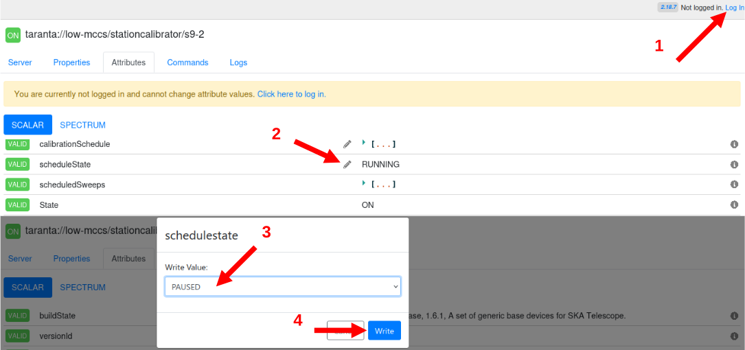Alternatively, it can be done through the Taranta web interface (Taranta). First login to Taranta, then find the relevant station calibrator device. Then click the pencil icon next to scheduleState to edit it. Then change it to PAUSED and click the “Write” button.

Using Calibration in Observations

If the calibration store has been set up correctly, then each station should have a “golden” calibration solution ready for use. For more information on MCCS calibration see the general calibration documentation or the calibration store documentation. The process for adding new calibration solutions to the store is described in Adding a new calibration to the store.

Alternatively, calibration solutions can be generated with the calibration SFT and saved as a numpy file. There are several functions for applying calibration solutions in aiv_utils.calibration_utils. In future, we will be able to apply solutions by using their name in the Configure step.

Applying Calibration in TMCObservation.ipynb

If you are using the TMCObservation.ipynb notebook, TMC will automatically apply this solution as part of the Configure command. The notebook also supports applying manual calibration and flagging of antennas.

If you want to apply manual calibration to at least on of the stations, set the CALIBRATIONS parameter. This parameter should be a list of strings that is the same length, and in the same order as the STATION_NAMES parameter. Each string can specify either a calibration method (e.g. "UNITY" to apply unity calibration), or a path to saved calibration solution in the standard [antenna, channels, pol] format. You can have a mix of calibration types, for example if STATION_NAMES = ["s8-1", "s8-6", "s9-2"] and CALIBRATIONS = ["FROM_STORE", "solutions/fitted_gain_solutions.npy", "UNITY"], then S8-1 will have the calibration from the calibration store applied, S8-6 will have the calibration solution located at solutions/fitted_gain_solutions.npy applied, and S9-2 will have a unity calibration applied. If the CALIBRATIONS parameter is not set, or is an empty list, then all stations will have solutions applied from the store.

Note

All stations will by default have solutions applied from the calibration store when Configure is called. The manual calibration step takes place between Configure and Scan to optionally overwrite the solutions that were automatically applied. There is no way for TMC to not apply any solution. If a solution is not found in the store, then a unity calibration is applied.

If you want to flag antennas (set their complex gain to zero so that they do not contribute to the beam), set the FLAGGED_ANTENNAS parameter to be a list of lists of antenna names (e.g. “sb11-02”) to flag. The list of lists should be the same length, and in the same order as the STATION_NAMES parameter. Specify an empty list to not flag any antennas in that station. For example, if STATION_NAMES = ["s9-2", "s10-3"] and FLAGGED_ANTENNAS = [[], ["sb11-01", "sb08-09"]], then no antennas will be flagged for S9-2, but the antennas in S10-3 with names sb11-01 and sb08-09 will have complex gain of 0 and any data coming from these antennas will not be included in the beam.

Applying Calibration in AcquireBeamformed.ipynb

When using the AcquireBeamformed.ipynb notebook, set CALIBRATIONS to be a list of calibrations that you want applied to each station. Each item in this list can either be a path to a calibration solution or one of the special strings listed below.

"FROM_STORE": the station’s “golden” calibration solution will automatically be applied.
"UNITY": unity calibration solutions will be used, that is, the complex gain for xx and yy polarisation will be 1+0i and the gain for xy and yx polarisation will be 0+0i.
"NONE": no calibration is applied and the previous calibration is used. This only works if the previous calibration solutions loaded were for the same observation channels. For example, if the station was previously calibrated for an observation starting at channel 204, you would not be able to do an observation starting at channel 140 without needing to first apply new calibration solutions.
"ZERO": zero amplitude calibration is applied to all polarisations so that no data comes out of the beam. This is likely only useful for testing purposes.

If using a saved calibration solution (e.g. from the calibration SFT), you need to set the calibration to the path to the .npy file. You can also specify the starting channel of the solutions with GAIN_SOLNS_START_CHANNEL. If the solution file has the shape [channels, antenna, pol], instead of the usual [antenna, channels, pol], then set the IS_CHANNELS_FIRST parameter to True. If you are using solutions generated by the calibration SFT, IS_CHANNELS_FIRST doesn’t need to be changed from its default value of False .

Antennas to be flagged (set their complex gain to zero so that they do not contribute to the beam) can be specified with the FLAGGED_ANTENNAS parameter. This parameter is a list of lists of antenna names.