Introduction

The following sections document the process developers should follow to improve and maintain the ska-low repository.

Contributing to the ska-low repository

To contribute to the ska-low repository, you should first create a Jira issue describing your work and the acceptance criteria. This ticket is used in the name of your branch and your commit message as described in the SKA developer docs. Once you have completed your changes and the tests pass, you can create a merge request and assign it to a reviewer. The Vulcan team will review your changes and merge them into the main branch if they are approved.

Testing

There are three major ways that we run tests:

Manual notebooks: Run the notebooks by going through the jupyter notebook cells, copy the result notebook to a separate directory and manually write the results to either Jira Xray or Jama. This is how we run the integration notebooks and some of the SFT notebooks.
run_notebooks: Run the notebooks using the run_notebooks script which wraps papermill. This is how we run the SFT notebooks and some of our regular frequency sweep observations.
pytest BDD: Run the tests using Behavior Driven Development (BDD) test descriptions and pytest. This is how we do most of our automated tests

Automated tests

Our testing is moving towards using pytest and Behaviour Driven Design (BDD) as much as possible. The types of tests we run are categorised by the marks we have given them. These categories are explained in later sections and include:

operations explained in Operational notebooks
tmc_scans explained in TMC notebooks
on_off_commands explained in On and off commands
health_roll_up explained in Health report and roll up
unit explained in Unit tests

All test categories except for unit are automatically run using a GitLab pipeline that launches at 2:00 a.m. if the ITF is available. We call this set our regression tests which is run using PYTEST_MARKERS="operations or tmc_scans or on_off_commands or health_roll_up". It generates an Allure HTML test report, which is included as part of the job, and uploads the results to Jira Xray under the Regression Test Plan.

The tests are written following this guide and are described in the tests/features/*feature files using the Gerkin syntax. These feature files are compiled into markdown descriptions using the ska-ser-xray generate-steps-docs command. The docs describe the high level features and the low level steps (which can help finding the code that executes each step). The bdd-test-docs-check GitLab pipeline job checks if these feature files are up to date. If they are not, then run this command:

generate-steps-docs tests/ tests/docs

And commit the changes.

Running the tests manually

The tests can be run manually in the JupyterHub terminal, from the ska-low repo directory (which is /home/jovyan/ska-low/ on Jupyterhub), using the following command:

make test

This will automatically run the pytest suite with some standard arguments and then generate an Allure HTML report from the results. This report will be output to a directory like ska-low/build/reports_2025-11-12_06-24-17/allure_report/index.html where the date and time is when the tests were run. You can download this file and open it in a web browser to view the results and attach it to SKBs.

Useful variables you can pass to the tests include:

STATIONS: A comma-separated list of station names to run the tests on. For example, to run the tests on stations itf1 and itf2, use STATIONS="itf1,itf2". By default all stations are used.
SUBARRAYS: A comma-separated list of subarray names to run the tests on. For example, to run the tests on subarrays 1 and 2, use SUBARRAYS="1,2". By default all subarrays are used.
PYTEST_MARKERS: A pytest expression to filter which tests to run. For example, to only run the operational notebooks tests, use PYTEST_MARKERS="operations".
TESTS_TO_RUN: The function name of the test to run. In the pytest stdout this will be the name to the right of the ::. For example, to only run the test named test_field_nodes_on from the tests/functional/test_station_operations.py file, use TESTS_TO_RUN="test_field_nodes_on".
NOTIFY: A flag to set a notification to be served on a printed URL. For example, to have a notification be served at the end of the test run, use NOTIFY="true". A unique link (looking like https://ntfy.sh/{A_UNIQUE_32_BIT_STRING}) will be printed during the start of the test run, which can be opened in a browser window. Make sure that the website has permission to show notifications (only needs to be done once). Once done, you can safely navigate away and a notification will appear when the test run ends.
ITF: A flag to quickly set the SUBARRAYS and STATIONS for either DEV stations or EM. For example, use ITF="EM" for itf3 & itf4 with subarray 1 & 2. Use "DEV" for itf1 & itf2 with subarray 3 & 4.
PARALLEL: A flag to run station tests in parallel (one station per thread). False by default and set to on with PARALLEL=true. Parallel runs will skip all TMC/multi-station tests until LOW-2409 is completed.

For example, if you want to run the full regression suite on the Dev ITF, you can run:

make test STATIONS="itf1,itf2" SUBARRAYS="3,4" PYTEST_MARKERS="operations or tmc_scans or on_off_commands or health_roll_up"

Or, this could also be

make test ITF="DEV" PYTEST_MARKERS="operations or tmc_scans or on_off_commands or health_roll_up"

Or if you want only to run the TMC notebook tests on the EM ITF, while being notified at the end, you can run:

make test STATIONS="itf3,itf4" SUBARRAYS="1,2" PYTEST_MARKERS="tmc_notebooks" NOTIFY="true"

Or if you want to run the operation notebooks (which don’t need a subarray) on the AA0.5 stations, you can run:

make test STATIONS="s8-1,s8-6,s9-2,s10-3" PYTEST_MARKERS="operations"

You can also run the station level tests in parallel (one station per thread) with PARALLEL=true and multiple times with PYTEST_OPTIONS="--count x" like so:

make test STATIONS="s8-1,s8-6,s9-2,s10-3" PYTEST_MARKERS="operations" PARALLEL=true PYTEST_OPTIONS="--count 20"

This command runs each test in operations 20 times for the stations s8-1, s8-6, s9-2, and s10-3 in parallel.

Running the tests using the GitLab pipeline

To ensure we everything we merge into main works, we should run the regression pipeline before merging into main. The tests only run manually. To launch the pipeline, click start/play on the job named “test:itf:regression”. This job will use the is_calendar_booked script to check the calendar and determine if the Dev ITF is booked and if it is not it will use station itf1 and itf2 to run the tests. If you have already booked the ITF and you know it is safe to run the tests, you can pass edit the variable CHECK_CALENDAR to false to skip the calendar check. For an example of how to do this, see the SFT Notebooks section below.

Operational notebooks

The operational notebooks are run using the operations pytest mark, described in the tests/features/station_operations_XTP-62364.feature file and written in the tests/functional/test_station_operations.py file. The majority of the tests are run by using papermill to execute the operational notebooks in notebooks/operations with different parameters and then checking the results. These are mostly running MCCS-level commands, so they can be thought of as station-level tests.

TMC notebooks

The TMC notebooks are run using the tmc_notebooks pytest mark, described in the tests/features/tmc_scans_XTP-75814.feature file and written in the tests/functional/test_tmc_scans.py file. These tests run the notebooks/operations/TMCObservation.ipynb notebook using papermill. These are considered end-to-end tests, as they test the full signal path from the tile to data capture. The different tests cover various types of observations (such as visibility and PST) in different ways (such as using multiple subarrays or beams simultaneously).

On and off commands

The on and off commands are run using the on_off_commands pytest mark, described in the tests/features/on_off_commands.feature file and written in the tests/functional/test_on_off_commands.py file. These tests move away from notebooks and use only Tango device commands to mimic how station operators and field techs plan to use the telescope.

Health report and roll up

The health tests are run using the health_roll_up pytest mark, described in the tests/features/station_health_roll_up.feature file and written in the tests/functional/test_station_health_roll_up.py file. These are often destructive tests that attempt to put the station or telescope into a degraded state to ensure that the health reports and roll-ups accurately reflect the telescope’s state. It also ensures that the telescope can recover from these bad states correctly. As part of the test clean up, the operational notebooks are used to return the station to a healthy state.

Unit tests

The unit tests are run using the unit pytest mark and written in the tests/unit directory. They are a limited number of unit tests for the aiv_utils module which can be run using:

pytest -m unit

SFT Notebooks

The Short Functional Tests (SFTs) are located in notebooks/SFT and are run per station when it is first being integrated or after maintenance to ensure it is working correctly. The results of these tests are stored in /home/jovyan/shared/test_executions and uploaded to Jira Xray under the Station SFTs Test Plan.

The SFT notebooks are currently run either manually, using the run_notebooks command or using a gitlab runner (which uses the run_notebooks command). When running the notebooks in this way, notebook outputs can be read by subsequent notebooks that are run as part of the same run_notebooks command. For example, the frequency sweep notebook will store the path to the captured data in an environment variable that is then used by the closure and calibration SFT notebooks. Similarly, the calibration SFT stores the path to calibration solutions that can be used by the sun drift SFT.

You can use run_notebooks -h to explain the command arguments. Some of the most useful ones are:

–station-name: the name of the station being tested
-p: Can be called multiple times to pass parameter key pairs to the notebook. For example: -p CALIBRATION_TYPE SUN_FAST -p CAPTURED_DATA_PATH /data/path.
–early-stop: don’t run subsequent notebooks if one has an error

The following are some examples of how to run the notebooks:

Run frequency sweep and calibration SFT:

run_notebooks --station-name s10-3 --early-stop -p CALIBRATION_TYPE SUN_FAST notebooks/SFT/03*/*.ipynb notebooks/SFT/06*/*.ipynb

For more information on running the calibration SFT see Calibration.

If you have already run the frequency sweep SFT or a manual frequency sweep, you can use this existing data in the calibration SFT using the CAPTURED_DATA_PATH parameter like so:

run_notebooks --station-name s10-3 -p CALIBRATION_TYPE SUN_FAST -p CAPTURED_DATA_PATH /home/jovyan/shared/test_executions/03.FrequencySweep/s10-3_2024-11-24_155157/captured_data notebooks/SFT/06*/*.ipynb

In a similar way you can use the existing data source and the CAPTURED_DATA_PATH parameter for the closure SFTs:

run_notebooks --station-name s10-3 -p CAPTURED_DATA_PATH /home/jovyan/shared/test_executions/03.FrequencySweep/s10-3_2024-11-24_155157/captured_data notebooks/SFT/04*/*.ipynb

Note

If the run_notebooks command should is run outside of the base ska-low directory, then you will need to specify absolute paths to the notebooks that you want to run. For example notebooks/SFT/06*/*.ipynb would need to be changed to /home/jovyan/ska-low/notebooks/SFT/06*/*.ipynb. For this reason, it is recommended to run cd ~/ska-low before using the run_notebooks script.

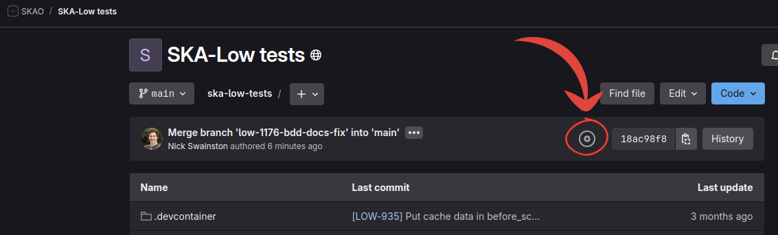
The SFTs can also be launched from the ska-low gitlab pipeline runners if you have at least “Developer” level access to the repository. You can launch the manual pipeline from any commit, but the best practice is normally to run it off the most recent main commit. To do this go to the ska-low repository and click on the pipeline status button:

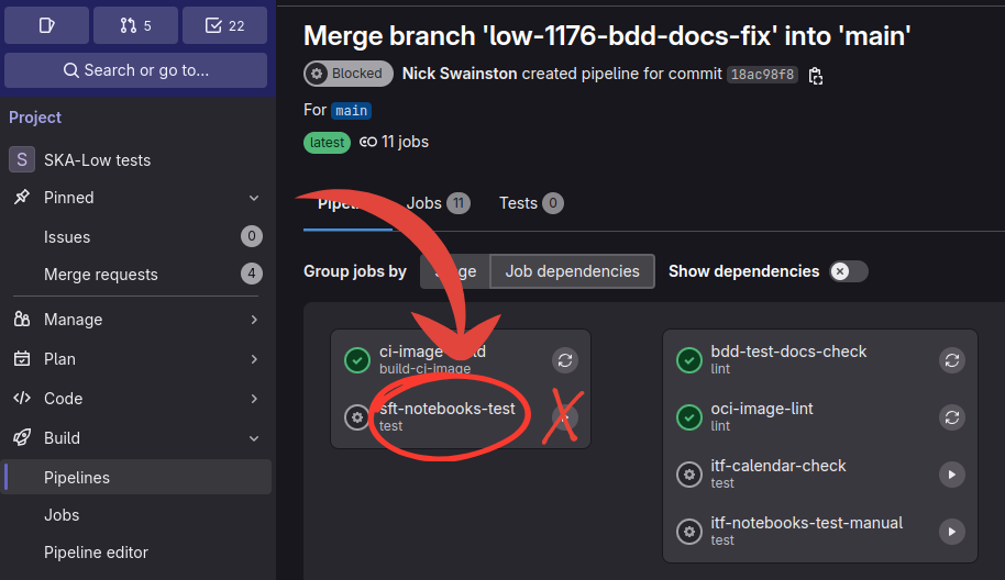
Then click on the text “sft-notebooks-test” and NOT the play button (this will launch the pipeline without parameters):

Then you can add the parameters in the “Variables” section. You must include the following variables:

STATION: the name of the station being tested
NOTEBOOKS: the notebooks to run
PARAMETERS: the parameters to pass to the notebooks

For example:

STATION: s9-2
NOTEBOOKS: notebooks/SFT/04*/*.ipynb notebooks/SFT/05*/*.ipynb notebooks/SFT/06*/*.ipynb
PARAMETERS: --early-stop -p CAPTURED_DATA_PATH path/to/data -p CALIBRATION_TYPE SUN

Which looks like this:

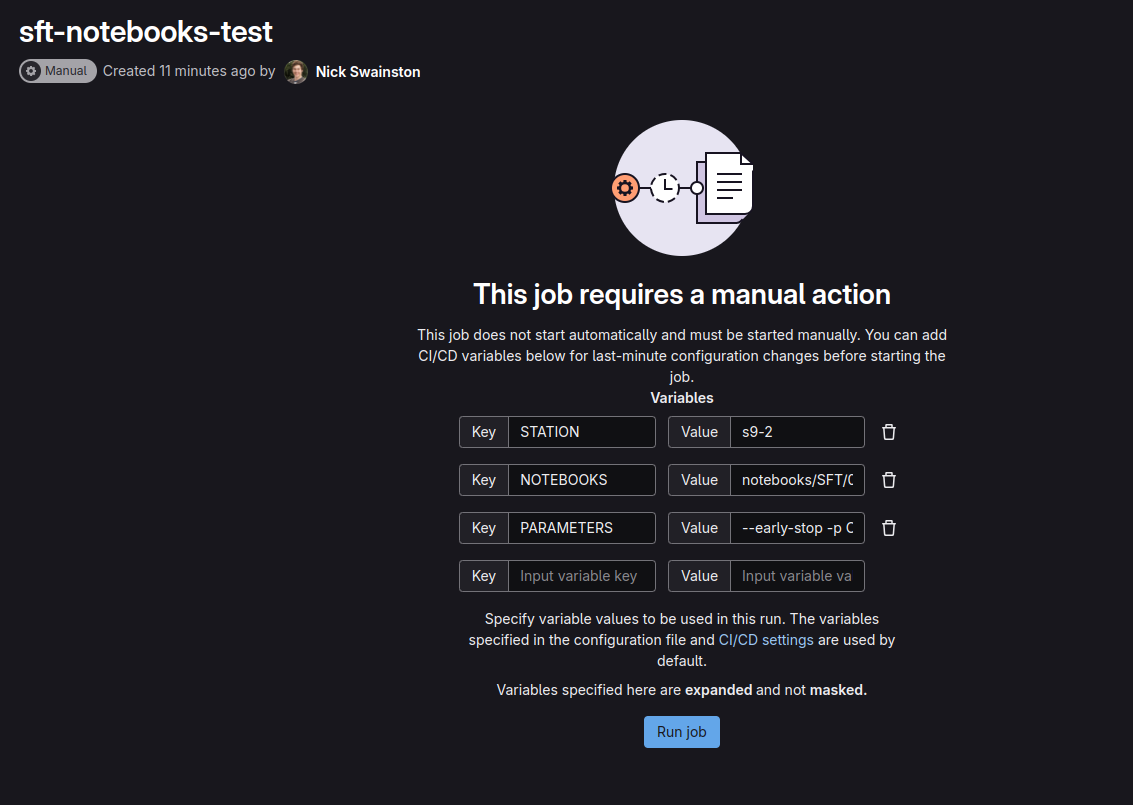
Then click run and you can watch the progress of the job and even relaunch it with updated parameters if needed.

Integration Notebooks

The integration notebooks are located in notebooks/integration and notebooks/ITF/integration and are only run manually. Their results are written to Jama and copies of the executed notebooks pushed to the ska-low-test-artefacts repository.

Publishing new chart versions

Publishing new ska-low, ska-low-skaffold and ska-low-dm chart versions is required to deploy the latest changes to the production clusters. Instructions on how deploy published charts are in the ska-low-deploy repository README.md.

When updating the chart dependencies in the Chart.yaml files, make sure you also update the Chart.lock file. You can do this by running the following command in the ska-low repository:

helm dependency update charts/<chart_name>

So for example to update the ska-low chart dependencies, you would run:

helm dependency update charts/ska-low

Then commit and push the changes to the ska-low repository.

Development versions

Every time a new commit is pushed, the gitlab pipeline will create a new development version of the chart. To find this version, got the pipelines page and find the pipeline for your commit. Wait for the helm-chart-build job to finish then click on it to view the logs. One of the final lines of the logs will be similar to:

helmChartBuild: publishing ska-low-26.2.0-rc4-dev.ccf197041.tgz

The text after ska-low- and before .tgz is the version of the chart. So in this above example the version is 26.2.0-rc4-dev.ccf197041 which can be used in ska-low-deploy repository’s helmfile.yaml.

Release versions

Using releases and changelogs to document software deployments on a cluster provides clear traceability and simplifies tracking changes and troubleshooting across environments. The intended release cadence is once-per-sprint, and versions are time-based, of the form <pi>.<sprint>.<patch>, such that the first release made in the first sprint of PI 26 is 26.1.0.

The Release Management (REL) Jira issues are generally created for all sprints at the start of the PI. Guidance and tooling for this are available in the REL/ folder.

Preparing for a release

To ensure a quality release, check the following things are up to date:

Run the todo_tracker
The output the status of the Jira tickets (such as SKBs) that we mention in our repo. Any workarounds for closed tickets should be removed and updated on the CHANGELOG.md file.
Ensure the docs are up to date.
If anything in the CHANGELOG.md is described in the documentation, then check if needs updating.
Publish the CHANGELOG.md to the team-low-aa1 Slack channel.
Try to do this two days before the release to give stake holders time to protest anything they don’t want to be deployed.

Making a release

Thanks to the prebump (see below), the chart and python versions should be up to date. You will need to update the vulcan images versions (everything we deploy using the containers in the images/ directory). They should all be marked with a TODO but you can also search for previous versions. Here is an example:

tag: 30.4.1  # TODO: Bump to 30.5.0 before tagging

This will work because once release the tag, these images will also be built.

Then update the CHANGELOG.md to include the date of the release:

## <version> - YYYY-MM-DD

E.g:

## 30.5.0 - 2026-05-29

Get the branch approved and merged on to main. From the main branch, locally run the following two commands to make the tag and push it:

make create-git-tag
make push-git-tag

You can then look at the Gitlab pipeline page to find the release/tag pipeline. Once the job helm-chart-publish is finished the chart is ready to be deployed.

Before deploying, first search for EMBARGOED in ska-low-deploy repo. The embargoed comments should explain what value changes are required before deploying. Once embargoed comments are removed or resolved, you can create a diff and sync if the diff looks correct.

Once deployed you should check the pods are all running and run our regression checks. Hopefully it will be that easy, good luck!

Clean up and preparing for the next release (prebumping)

To keep the dev version format like a release candidate for a future version, we prebump the version after a release. Grab the REL ticket for the next release (normally on the Miro board) and make a MR with the following changes.

The process for bumping versions of the ska-low, ska-low-skaffold and ska-low-dm charts is the standard process as outlined in the developer portal; see How to make a release. Normally we will be doing a minor bump for the next sprint.

Once the versions of the charts are bumped you will need to update the Chart.lock with:

helm dependency update charts/<chart_name>

Update the CHANGELOG.md to include the the prebumped version and the changelog format like so:

## <version> - Unreleased

### Added

### Changed

#### Version updates

### Fixed

### Removed

Add comments to the values of the our image versions (everything we deploy using the containers in the images/ directory) like so:

tag: 30.4.1  # TODO: Bump to 30.5.0 before tagging

Here is an MR as an example.

Deployment

Vulcan uses the ska-low-deploy repository to deploy the SKA-Low software to the production clusters (North MCCS and South Pawsey) and to the Low-ITF. This repository contains the helmfile and helm charts that can use the telmodel data to deploy the required software to the kubernetes clusters.

The ska-low-deploy repository has a README.md which explains how to deploy the software. The deployed versions can be seen on the Deployment details (ITF, Low AA) dashboard in Grafana.

Grafana Dashboards and the EDA database

To monitor current and historical data of the SKA-Low telescope’s state, we use Grafana dashboards. Grafana simply queries a database and presents the data graphically in a dashboard so it can be easily understood. This database is populated continuously by recording the attributes of Tango devices that we consider important. The following sections will explain how to use and improve the database (The Database (EDA)) and the dashboards (Grafana).

The Database (EDA)

The Engineering Data Archive (EDA) is a database that stores the historical data of the SKA-Low telescope. The EDA is a PostgreSQL database that is deployed on the SKA-Low (north and south) and the ITF. You can access the EDA database using python (in JupyterHub) or through database tools like pgAdmin.

Accessing the EDA using JupyterHub

To query the EDA database through JupyterHub, log into the the cluster of the EDA you wish to query (you can access the North MCCS EDA from the North MCCS JupyterHub). Then, you can use the following code to query the database:

import os
import pandas as pd

# Check you have the right environment variables to give you access permissions
print("\n".join(f"{k} = {v}" for k, v in os.environ.items() if k.startswith("PG")))

# Use pandas to make the query and display the results
df = pd.read_sql_query(
    """
    SELECT
        data_time,
        member,
        value_r
    FROM
        scalar_devstring
    where
        quality = 0
        and name = 'tileprogrammingstate'
        and member in ('s9-2-tpm01','s9-2-tpm02','s9-2-tpm03')
        and data_time BETWEEN '2025-01-20T02:50:55.764Z' AND '2025-01-20T02:55:55.766Z'
    order by 1;
    """,
    "postgresql+psycopg://",
    params=('a parameter', 42, ["A", "B", "C"])
)
display(df)
display(df.dtypes)

To understand the schema used in the above query, see the Database Schema section. This code and more examples can be found in the notebooks/examples/EDA_example.ipynb file in the ska-low repository. You can follow along in the examples in the notebook (which have similar explanations to this document) to learn how to query the database.

Accessing the EDA using pgAdmin

Tools like pgAdmin can be used to query the database using SQL queries. To connect to the EDA database using pgAdmin, you need to create a new server connection with the following details:

Connection: Host name/address:

North MCCS: eda.ska-tango-archiver.svc.mccs.low.internal.skao.int
South Pawsey: eda.ska-tango-archiver.svc.low.internal.skao.int
ITF: eda.ska-tango-archiver.svc.lowitf.internal.skao.int

Maintenance database: eda

Username: eda_ro

Password: Copy the password from the PGPASSWORD environment variable in the JupyterHub terminal.

Once you have connected to the EDA database, you can run SQL queries to retrieve data from the database. See the Database Schema section for more information on the database schema and the Query Examples section for examples of SQL queries you can run.

Archivers

The database must be populated with data from the Tango devices, which is done by the ska-low-tango-archiver subchart. Archiving configuration lives in charts/ska-low/values.yaml under the ska-low-tango-archiver key, split between classDefaults (per-class attribute archiving configs, defined once and reused) and configuration (grouped into one ConfigMap per entry, each applied to HDB++).

For example:

ska-low-tango-archiver:
  classDefaults:
    MccsController:
      state: { archive_period: 5000, polling_period: 5000 }
      adminMode: { archive_period: 5000, polling_period: 5000 }
      healthState: { archive_period: 5000, polling_period: 5000 }
      healthReport: { archive_period: 5000, polling_period: 5000 }

  configuration:
    mccs-control:
    - db: "{{ .Values.global.tango_host }}"
      manager: low-eda/cm/01
      archiver: low-eda/es/01
      configuration:
        - class: MccsController  # attributes substituted from classDefaults

This configures archiving for the MccsController Tango device to record the state, adminMode, healthState and healthReport attributes every 5000 ms (5 seconds). To record additional attributes, add them to the MccsController entry under classDefaults with an appropriate archive_period and polling_period. A configuration entry that supplies its own attributes block is used as-is (no merging with the defaults). Members of the Vulcan team can help to deploy changes to the archiver configuration, or you can follow the “how to deploy the software” guide.

Database Schema

The tables that the archivers use have the name format <major_data_type>_dev<minor_data_type> where <major_data_type>_ is either scalar, array, image or conf and <minor_data_type> is either boolean, double, encoded, enum, float, long, string, etc. So health reports for example are strings and are written to the array_devstring table and the array of 4 subrack fan speeds for the FNDH are in array_devdouble. The tables have a large number of columns but the most important ones are:

data_time: The time the data was recorded with timezone information.
value_r: The actual data recorded.
member: The name of the Tango device (e.g. "s9-2-sb16").
family: The family or type of the Tango device (e.g. smartbox).
domain: The domain or namespace of the Tango device (e.g. low-mccs).
name: The name or attribute of the Tango device that is recorded (e.g. adcpower).

You can use these columns to filter down to only the devices and attributes you are interested in.

To work out which table is used for the attribute you are interested in, the following query can be used to list all attributes recorded for a single device and their table:

SELECT
    distinct name,
    table_name
FROM
    att_conf
WHERE
    family = 'smartbox'
    AND member = 's9-1-sb01'

In this example we are looking for all the attributes of the smartbox family for the s9-1-sb01 device, but change it to the device you are interested in.

Query Examples

You can find examples of the queries by looking at similar panels in the Grafana dashboards, clicking edit and inspecting the query. For example the TPM tileProgrammingState query in the SPS dashboard is:

SELECT
    $__timeGroup(data_time, $__interval, NULL),
    member metric,
    (select val from tpm_states where name = (mode() within group (order by value_r)))
FROM
    scalar_devstring
where
    quality = 0
    and name = 'tileprogrammingstate'
    and member in ($tpm)
    and $__timeFilter(data_time)
group by 1, 2
order by 1;

Two common things to note in the queries are the $__timeFilter(data_time) and the $__timeGroup(data_time, $__interval, NULL). The $__timeFilter(data_time) is a Grafana macro that filters the data to the time range selected in the Grafana dashboard. The $__timeGroup(data_time, $__interval, NULL) is a Grafana macro that groups the data by the time interval selected in the Grafana dashboard, this can be found under “Query options” and is best set to the same value as the polling_period. If you run these queries in pgAdmin, you will receive an error as the tools won’t know what these functions are. To convert this into something you can use, click on “Query inspector” and click “Refresh” and it should display the query with the macros expanded, including Variables like $tpm:

SELECT
    time_bucket('15.000s',data_time) AS "time",
    member metric,
    (select val from tpm_states where name = (mode() within group (order by value_r)))
FROM
    scalar_devstring
where
    quality = 0
    and name = 'tileprogrammingstate'
    and member in ('s9-2-tpm01','s9-2-tpm02','s9-2-tpm03','s9-2-tpm04','s9-2-tpm05','s9-2-tpm06','s9-2-tpm07','s9-2-tpm08','s9-2-tpm09','s9-2-tpm10','s9-2-tpm11','s9-2-tpm12','s9-2-tpm13','s9-2-tpm14','s9-2-tpm15','s9-2-tpm16')
    and data_time BETWEEN '2025-01-20T02:50:55.764Z' AND '2025-01-20T03:50:55.766Z'
group by 1, 2
order by 1;

You can also use this as an example of how to replace datetime and other variables in the query. Another common query is how we use unnest to unpack arrays, for example the TPM preADU attenuation query:

SELECT
    $__timeGroup(data_time, $__interval, NULL),
    to_char(adc_id, 'fm00') AS metric,
    mode() within group (order by adc)
FROM
    array_devdouble,
    unnest(value_r) with ordinality as t(adc, adc_id)
WHERE
    name = 'preadulevels'
    AND family = 'tile'
    AND member = '${tpm}'
    AND $__timeFilter(data_time)
GROUP BY 1, 2
ORDER BY 1

The unnest(value_r) with ordinality as t(adc, adc_id) line is used to unpack the array of values into separate rows with the adc_id column being the one based index of the array and adc the values. The adc values can then be used to get the mode (or the average in other cases) of the values in the array with mode() within group (order by adc). The adc_id is used in to_char(adc_id, 'fm00') to give it a leading zero and AS metric to label the row as what Grafana will use by default to label panels.

Grafana

The Grafana dashboards graphically display data from several data sources, most commonly the EDA database. An overview of the deployed dashboards can be found in the Homepage dashboard. If there isn’t a dashboard that covers your needs, or you would like to discuss dashboard improvements, please post a message on the #team-vulcan Slack channel.

When logged in with SKAO Entra, we can edit and create dashboards. Some of the dashboards directories with the ⇌ symbol are “provisioned” by Git Sync. Making changes to these dashboards have to be done through the Git Sync flow, which is explained in the Uploading changes section. For experimental development purposes, you can create personal dashboards in the Scratch folder (explained in section Creating Dashboards). This is not managed by Git Sync so it is vulnerable to data loss.

The following sections will explain how to create and improve the dashboards.

Creating Dashboards

To prevent clutter and so we can tell whose dashboard is whose, it is best to create dashboards in your own folder under the “Scratch” folder. Do this by clicking on “Scratch” on the dashboards page, then “New”, select “New folder” and give it your name.

When logged in with SKAO Entra, you can create a new dashboard by clicking on the “New” icon on the right side of the screen and selecting “New dashboard”. If you would like to keep creating it from scratch, first remember to save it by clicking “Save dashboard” and putting it into your personal directory. You can also duplicate an existing dashboard by clicking “Export”, “Export as code”, then “Copy to clipboard”. In your new dashboard, click “Import dashboard”, paste the JSON, and click “Save”. Then make sure you change the directory and the UID to something unique to avoid conflicts with the original dashboard.

One of the first things that are useful are setting up Variables which allow you to filter the data displayed on the dashboard. To create a new variable, click on the “Settings” icon on the right side of the screen and select “Variables”. Then click on the “Add variable” button and fill in the query which will find the variable.

A common variable is the station variable which can be created with the following query:

SELECT DISTINCT member FROM scalar_devstate WHERE family = 'spsstation' AND \$__timeFilter(data_time)

You can press “Run query” to confirm that the query is working and then “Back to list” when you are done.

Another important Grafana feature is the ability to Repeat rows and panels. This allows us to repeat a row for each station (like in the station overview dashboard) or a panel for each TPM (like in the SPS dashboard). This is also an important thing to understand when editing dashboard because you must edit the first row or panel to effect the rest.

Creating Panels

To create a panel, click “Add” then “Visualization” and select the type of panel you want to create. If you plan to make this a repeating panel, click “Repeat options” and add the variable you want to repeat on. You can then use this variable with the ${variable_name} syntax in the query to filter the data to the selected value.

At the bottom window you can edit you query but switching to “Code” mode and editing the query similar to the examples in the Query Examples section. You can also use the “Query inspector” to see the expanded query with the variables replaced with their values and the output of your query. You can use this to debug your query and to inform what “Value mappings” you should add to colour and edit the display of your panel. For example, we use value mappings to convert health state indexes to the health state names and a colour to reflect the severity of the health state.

Uploading changes

To create a new dashboard, you must save the dashboard in the new v2 YAML format. You can do this by clicking the “Export” button (in the right panel, with the arrow pointing down into a box), then selecting “Export as code”. Click the “Advanced options” drop-down and click “YAML”. You can then click “Copy to clipboard” and paste to a file in the resources/dashboards directory. You can then make a merge request with a link and screenshot of your dashboard so it can easily be reviewed and approved.

You can make changes directly on the provisioned dashboard with the Git Sync flow method. When you click save, you will be prompted to create a new branch and add a comment (a commit message) which you should link to a Jira ticket using the SKAO syntax. Once you have clicked save, you can click on the “Open pull request in Git” button. This won’t successfully make an MR for you but will take you to the right repository where you can create an MR with the branch you created.