Performance
Scaling
Algorithm 2 alternates between forming linear normal matrices for unknown, residual errors in the calibration model (station-based Jones matrices), and solving the normal equations to update the calibration model.
Algorithm 1 uses the fact that, for a large number of free parameters, the normal matrix is approximately block-diagonal with separate blocks for separate stations. As such, an approximation of the linear update at each iteration can be carried out separately for each station, with far fewer operations than algorithm 2. While algorithm 1 may take more iterations to converge, each one is faster and the overall runtime can be much lower. Particuarly when the number of free parameters is large.
The figure below demostrates runtime for three solver options, as implemented in this library. Algorithm 1 runtimes with default options are given in the left-hand panel, algorithm 2 runtimes with default options are given in the centre, and algorithm 2 runtimes with accum_opt 1 are given on the right. The tables below the figure show runtimes in finer detail as the number of iterations is increased from one. Typical solutions may take 10 - 20 iterations, unless starting from existing values such as those from a previous time step or frequency.
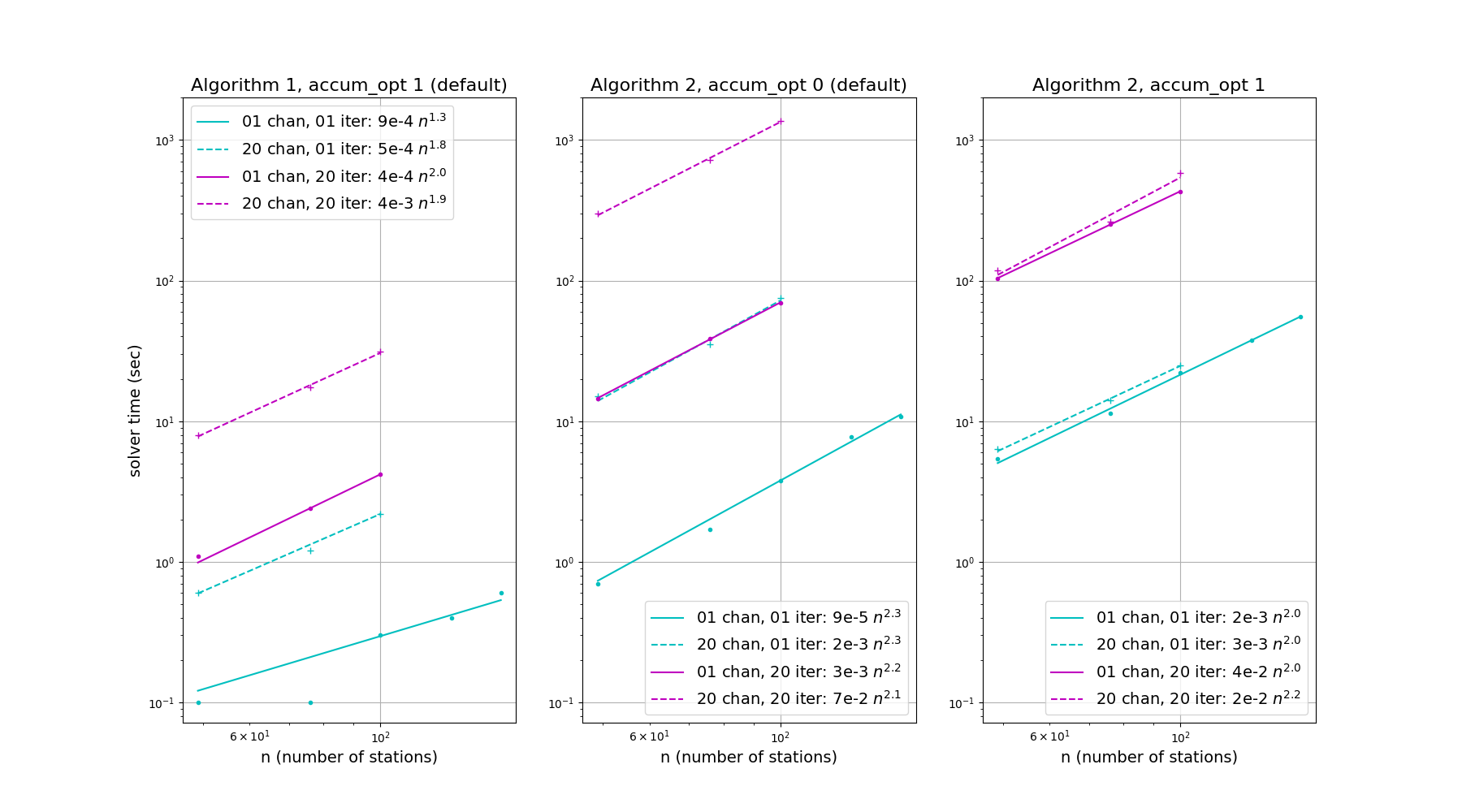
Algorithm 1, accum_opt 1, shows the shortest solver times, which scale with the number of free parameters squared. Runtime is dominated by a pass over the dataset during each iteration, and as such scales approximately linearly with the number of time and frequency samples, and with the number of iterations. Each pass over the data could be made parallel in various ways (such as time, frequency, antenna), but once per iteration the various 2x2 accumulation matrices need to be gathered to a central solver process for each time-frequency solution interval. There is also scope for avoiding full passes over the dataset during each iteration, in a similar manner as accum_opt 1 of algorithm 2, depending on the commutation properties of the Jones matrices (for instance, depending on whether the calibration errors occur on the left or right of the primary beam Jones matrix). This option may be added in the future.
Algorithm 2, accum_opt 0, forms the design matrix, \(A\), and data vector, \(r = vis-model\), once per iteration, and so, like algorithm 1, shows linear scaling with the number of time and frequency samples and the number of iterations. Scaling with the number of free parameters is more complicated. The accumulation of normal equations should scale roughly with the number of parameters squared – with various parallelism options, as in algorithm 1 – however solving the system of equations scales more rapidly and is less trivial to parallelise.
Algorithm 2, accum_opt 1, accumulates the \(A^HA\) and \(A^Hr\) matrices directly, but factorises them into products with coefficients that can be pre-summed before the iteration. While it can be seen that this is more time consuming than accum_opt 0 when the number of time and frequency samples is small – as may be the case for real-time calibation – runtime is much more stable as the number of time and frequency samples grows, thanks to the pre-summing. Like accum_opt 0, the accumulation process has various parallelism options. In Yandasoft, separate equations are formed in parallel across frequency and spectral Taylor term, before merging to a joint solver.
solver 1, accum_opt 1 |
solver 2, accum_opt 0 |
solver 2, accum_opt 1 |
|
|---|---|---|---|
niter = 1 |
0.1 sec |
1.7 sec |
11.4 sec |
niter = 2 |
0.2 sec |
3.6 sec |
22.7 sec |
niter = 3 |
0.3 sec |
5.5 sec |
35.6 sec |
solver 1, accum_opt 1 |
solver 2, accum_opt 0 |
solver 2, accum_opt 1 |
|
|---|---|---|---|
niter = 1 |
1.2 sec |
35.2 sec |
14.0 sec |
niter = 2 |
2.0 sec |
73.4 sec |
26.9 sec |
niter = 3 |
2.8 sec |
102.0 sec |
37.7 sec |
solver 1, accum_opt 1 |
solver 2, accum_opt 0 |
solver 2, accum_opt 1 |
|
|---|---|---|---|
niter = 1 |
2.3 sec |
69.0 sec |
16.4 sec |
niter = 2 |
3.9 sec |
141.9 sec |
31.7 sec |
niter = 3 |
5.3 sec |
201.2 sec |
42.6 sec |
Solutions
Here, algorithm 1, most suitable for RCAL, is compared with Algorithm 2. For this the SKA-LOW sensitivity calculator
described in Sokolowski et al. 2022, PASA 39 was used to calculate the
visibility noise level for the MWA EoR0 field at RA = 0 hrs, Dec = -27 deg. All tests were carried out using modified
versions of example script examples/scripts/run_AA0.5.py.
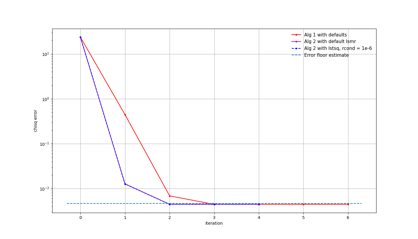
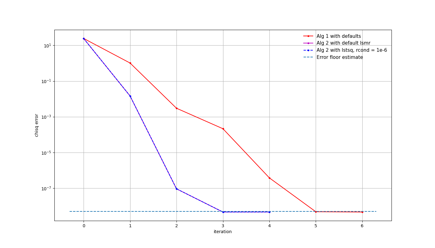
Creating a sky model from a single, strong (100 Jy) point source in the centre of the field, all solvers and seen to generate equivalent solutions. The following figure shows the \(\chi^2\)-error for three different solver options, with an array formed from 50 random stations from SKA-LOW and a simple Gaussian beam model. The calibration solution interval was set to 10 seconds and 10 MHz, which may be reasonable for real-time calibration of LOW during early array releases. The reason for including two versions of algorithm 2 will become apparent shortly. While it takes algorithm 1 more iterations to reach the expected noise level, the runtime was 1-2 seconds, rather than 30.
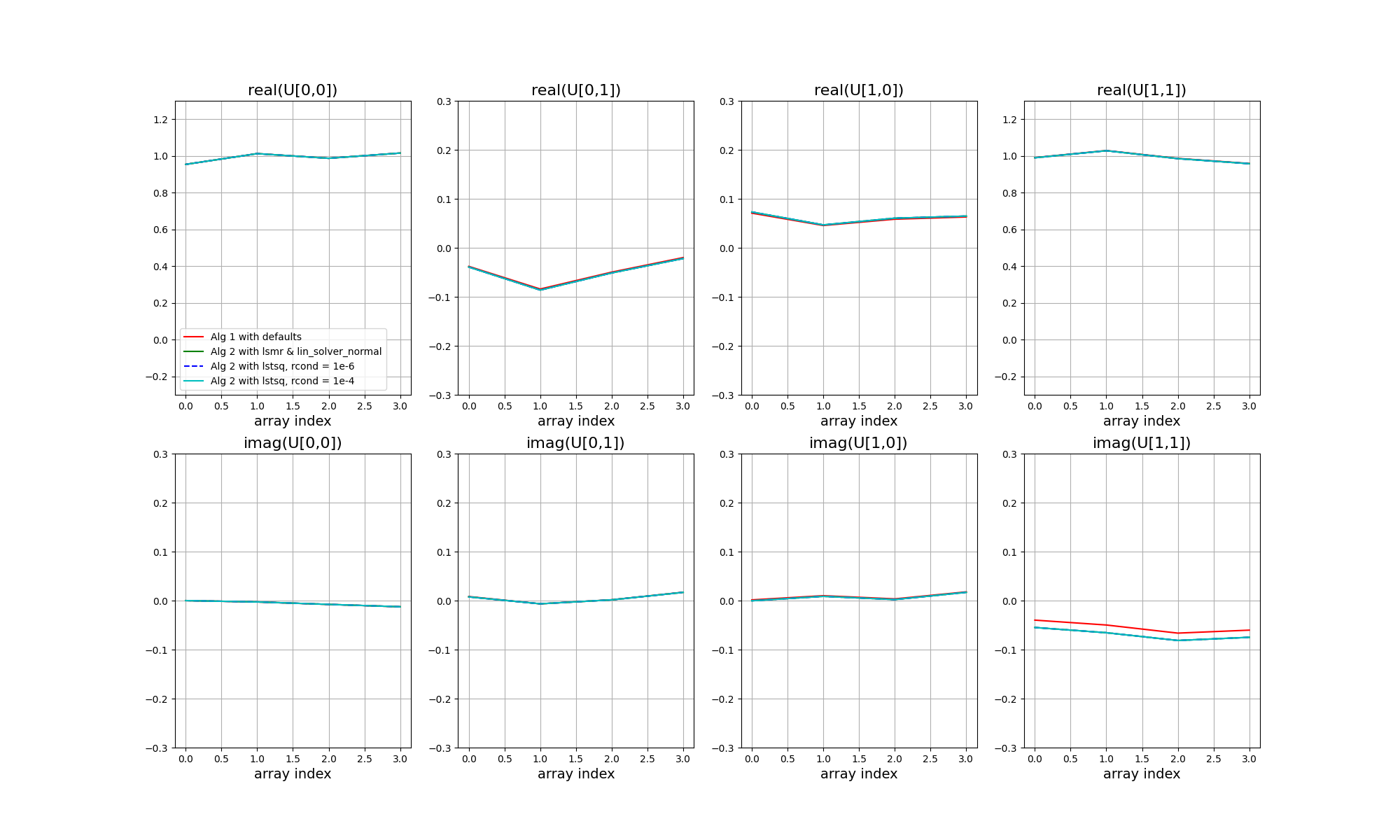
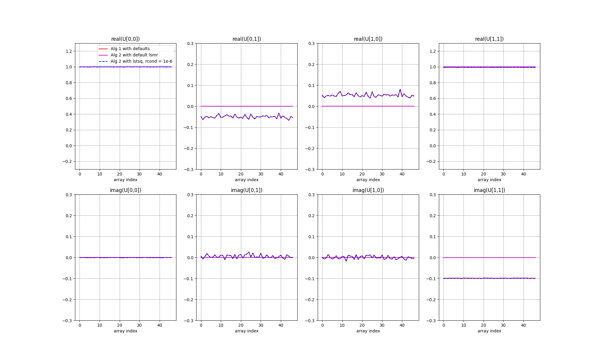
The next figure shows the solutions as coloured curves, relative to the input unknown Jones matrices in black. Each panel shows a different Jones matrix element, top panels real, bottom panels imaginary, with station index along the x axis. All data points have been phase referenced to the X polarisation receptor diagonal element of station 0.
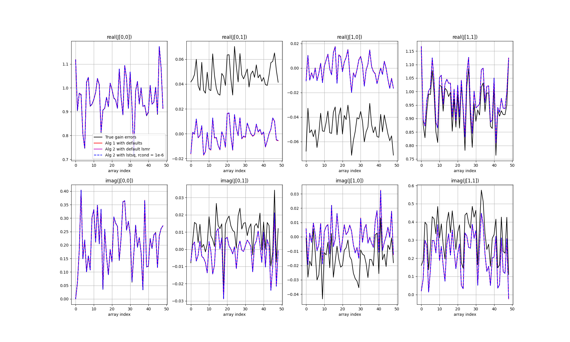
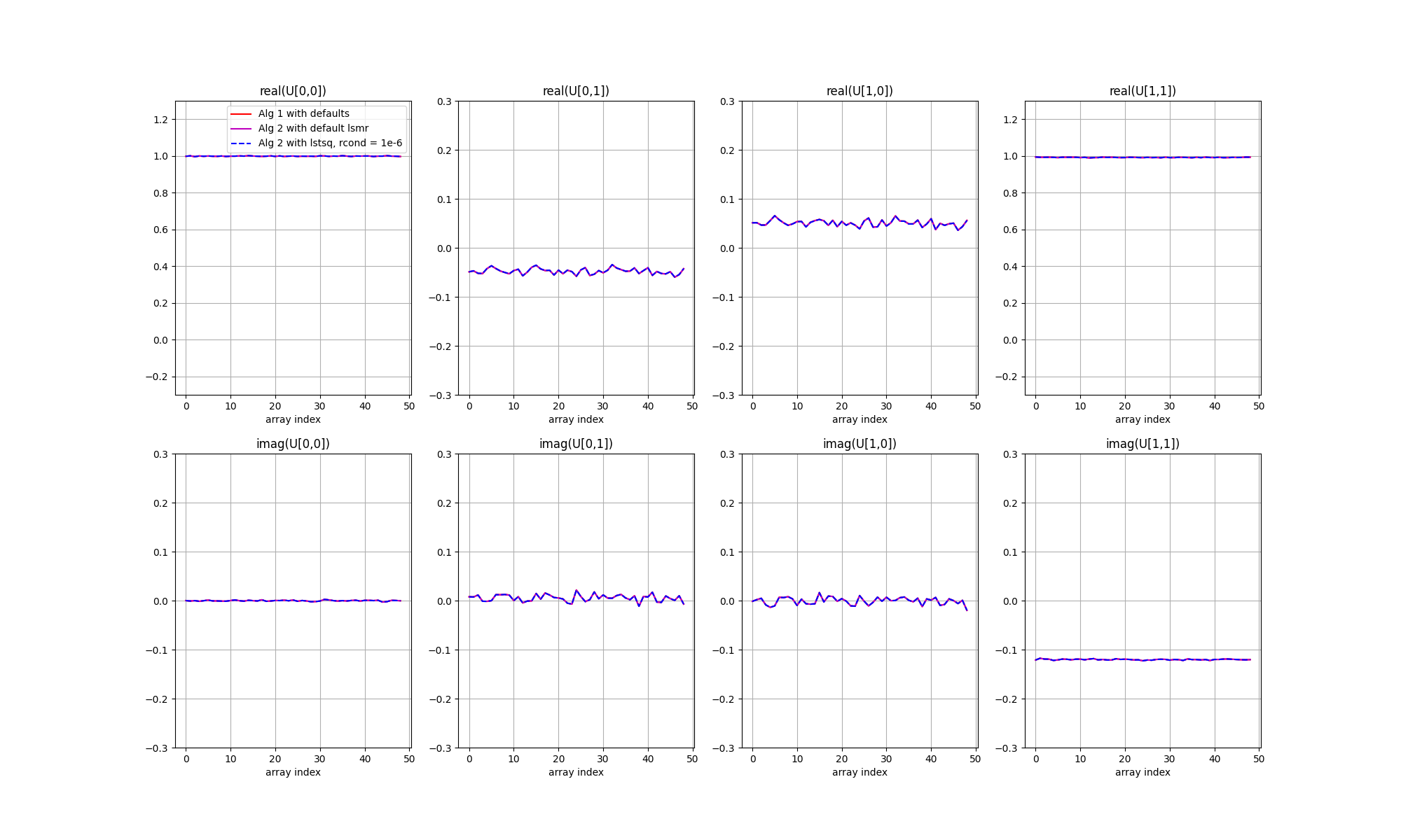
A few points to note. First, all three solvers result in the same solutions. However, there are offsets relative to the true values. This is more evident in the next figure, in which each solution matrix has been multiplied with the inverse of the true matrix. For ideal calibration the result would be 2x2 identity matrices, plus some noise. However a single, unpolarised cailbrator cannot constrain all of the unknowns, and ambiguities remain.
In the simulation, the input unknown Jones matrices comprised complex Gaussian random errors plus a systematic offset between the phase of the X and Y polarised receptors that was common to all stations, and systematic leakage between the receptors that was also common to all stations. The effect of XY-phase is seen as an offset from zero for the imaginary part of the Y diagonal term (noting that the phases have been referenced against the X receptor), and the effect of the leakage is seen as an offset from zero for the real part of the cross terms. The solutions have the expected form, and the separate polarisations are seen to be well calibrated.
If the noise is lowered, by adding more time or frequency samples, or more stations (or in this case by fudging the noise level in the simulation), the \(\chi^2\)-error improves, but these ambiguities remain.
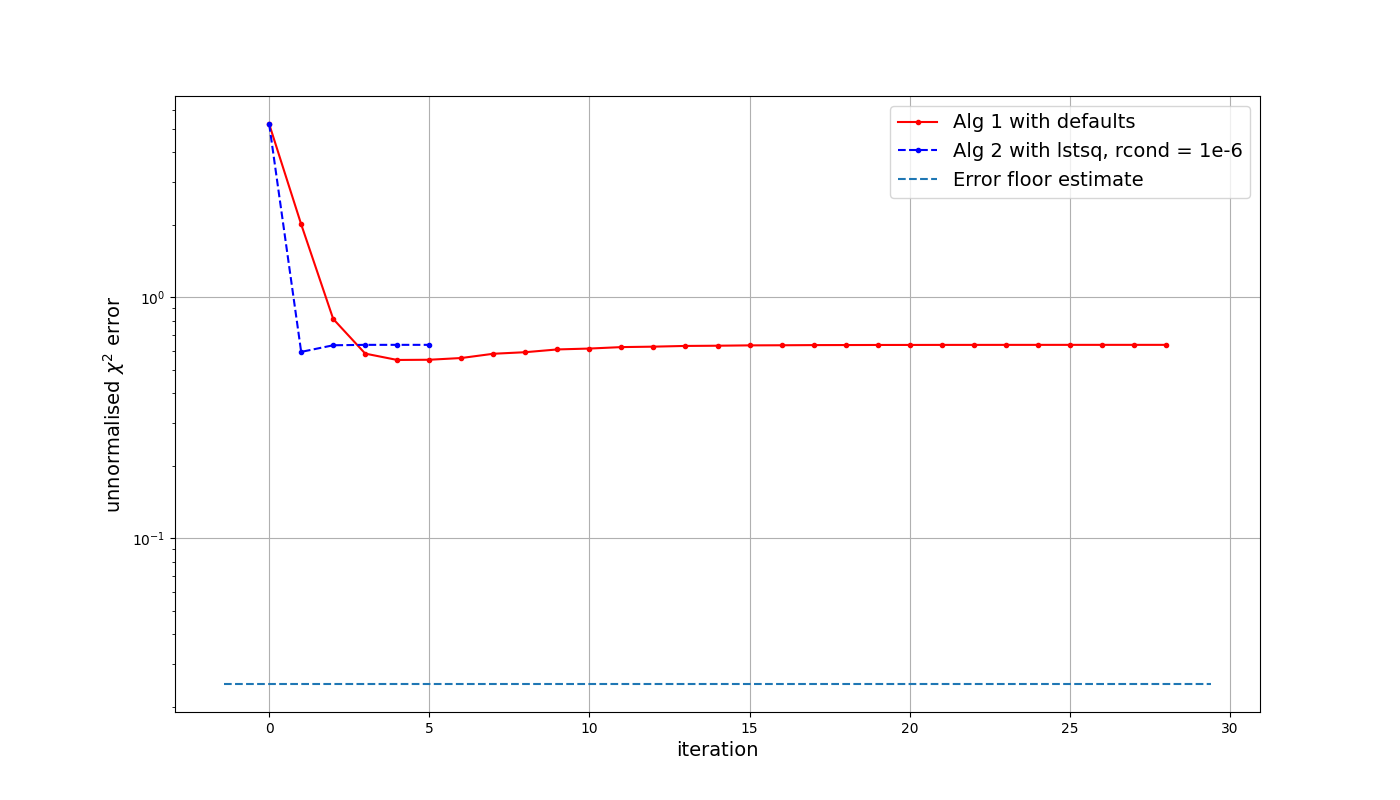
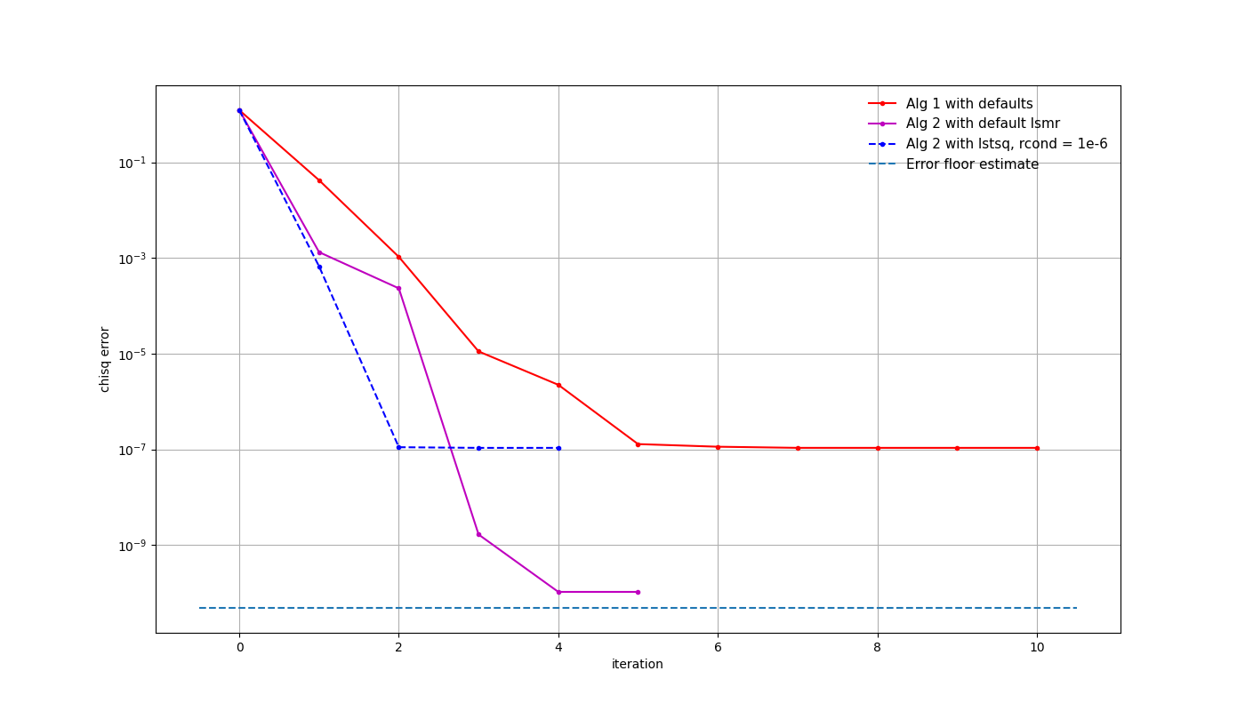
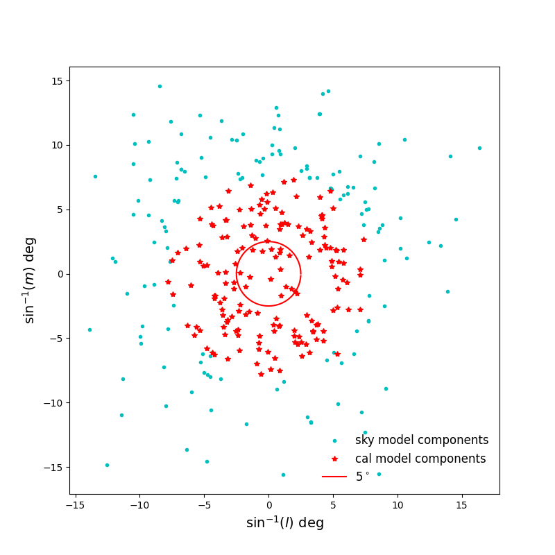
If we now replace the sky model with something more complex, such as the strongest 300 sources within 15 degrees of the EoR0 field, things look a bit different. Processing again with the high signal-to-noise ratio and the complete sky model, we see that the LSMR solver without the rcond cutoff performs better, while the other solvers hit a limit above the expected error level.
Looking at the calibration solutions, we can see that not only are the separate polarisations calibrated to a high accuracy, the ambiguities are also reduced. This is because of the extra polarisation information contained in the calibration model, coming from the instrument. It should be noted that it only performs at this level in high signal-to-noise situations, where factors like singular-value cutoffs can be set very low. If the noise level is high or the calibration model is incomplete, ambiguities start to grow. This aspect of the solvers is under active investigation.
Small Ararys
A similar simulation was run for a four-station AA0.5 array and the initial realistic noise levels, with a slightly longer calibration solution interval of 30 seconds to decrease the noise level a little. Again the EoR0 field with 300 sources was used in the simulation, but to generate some sky model errors, only components with an apparent flux density of 1 mJy were included in the calibration model.
The \(\chi^2\)-error shows some convergence, but the solutions hit a local minimum before reaching the expected error level. Nevertheless, the solutions are improved and coherent calibration is achieved for this quiet field without a dominant calibrator.