Diagnostic Data Products

This page describes diagnostic data products generated by the pipeline.

RFI Flagging Report

The RFI Flagging Report summarises the fraction of visibility data flagged as radio-frequency interference in each output dataset, across time, baseline, and frequency. Reports are saved as xarray datasets, which are self-descriptive collections of labeled multi-dimensional arrays that share dimensions and coordinate axes.

For each input visibility dataset, a corresponding report is saved in the main pipeline output directory as <INPUT_NAME>_flagging_report.zarr.

A corresponding plot of the report is saved as a PNG file as <INPUT_NAME>_flagging_report.png.

Standalone CLI app

It is also possible to generate a flagging report for any Measurement Set independently of the main pipeline, using the ska-sdp-flagging-report command:

ska-sdp-flagging-report path/to/dataset.ms

This saves dataset_flagging_report.zarr and dataset_flagging_report.png in the current working directory. The app uses a local Dask cluster sized to the number of available CPU cores.

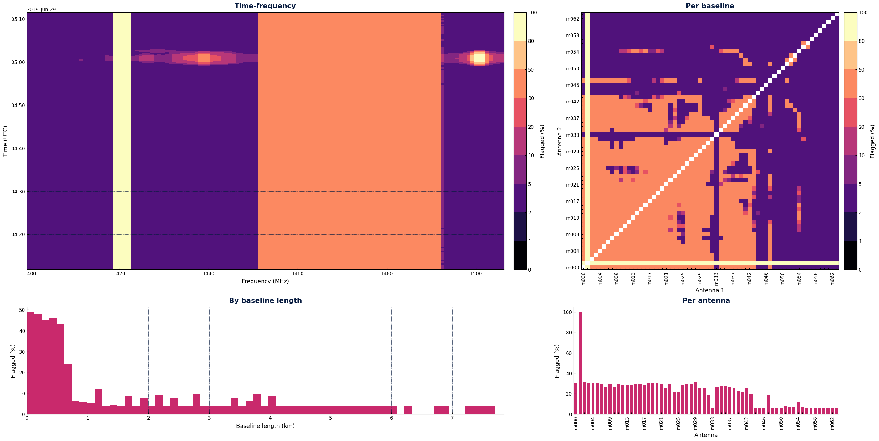
Example Plot

Here is an example plot of a flagging report as saved by the pipeline, after a run on a small MeerKAT dataset. Note that you can generate your own plots from the xarray dataset, see below.

Loading and working with reports

All you need is the xarray library to load and inspect flagging reports. For example:

import xarray as xr

report = xr.open_zarr("mydataset_flagging_report.zarr", chunks=None)
print(report)

This should print something similar to:

<xarray.Dataset> Size: 3MB
Dimensions:                 (baseline_id: 1953, frequency: 64, time: 224)
Coordinates:
    baseline_antenna1_name  (baseline_id) <U4 31kB ...
    baseline_antenna2_name  (baseline_id) <U4 31kB ...
* baseline_id             (baseline_id) int64 16kB 0 1 2 3 ... 1950 1951 1952
* frequency               (frequency) float64 512B 1.4e+09 ... 1.505e+09
* time                    (time) float64 2kB 5.068e+09 5.068e+09 ... 5.069e+09
Data variables:
    BASELINE_LENGTHS            (time, baseline_id) float64 3MB ...
    SUMS_BY_TIME_BASELINE       (time, baseline_id) int64 3MB ...
    SAMPLES_BY_TIME_BASELINE    (time, baseline_id) int64 3MB ...
    SUMS_BY_TIME_FREQUENCY      (time, frequency) int64 115kB ...
    SAMPLES_BY_TIME_FREQUENCY   (time, frequency) int64 115kB ...

You can easily access the data variables and coordinates by name. For example:

import matplotlib.pyplot as plt
import numpy as np

sums = report.SUMS_BY_TIME_BASELINE.values
samples = report.SAMPLES_BY_TIME_BASELINE.values
frac_by_time = np.nansum(sums, axis=1) / np.nansum(samples, axis=1)
plt.plot(report.time, frac_by_time)
plt.xlabel("Time (JD seconds)")
plt.ylabel("Fraction Flagged")
plt.show()

Data Schema

The RFI Flagging Report xarray dataset contains the following coordinates and data variables:

Coordinates

Name	Dimensions	Data type	Description
`time`	`[time]`	`float64`	Timestamp in JD seconds (CASA convention).
`baseline_id`	`[baseline_id]`	`int64`	Baseline unique ID.
`frequency`	`[frequency]`	`float64`	Channel centre frequencies in Hz.
`baseline_antenna1_name`	`[baseline_id]`	`str`	Antenna name for 1st antenna in baseline.
`baseline_antenna2_name`	`[baseline_id]`	`str`	Antenna name for 2nd antenna in baseline.

Data Variables

Name	Dimensions	Data type	Description
`BASELINE_LENGTHS`	`[time, baseline_id]`	`float64`	Projected baseline length in metres for a given (time, baseline) pair. NaN for (time, baseline) pairs absent from the data.
`SUMS_BY_TIME_BASELINE`	`[time, baseline_id]`	`int64`	Number of flagged visibility samples for a given (time, baseline) pair, summed across frequency and polarisation.
`SAMPLES_BY_TIME_BASELINE`	`[time, baseline_id]`	`int64`	Total number of visibility samples for a given (time, baseline) pair, summed across frequency and polarisation.
`SUMS_BY_TIME_FREQUENCY`	`[time, frequency]`	`int64`	Number of flagged visibility samples for a given (time, frequency) pair, summed across baselines and polarisation.
`SAMPLES_BY_TIME_FREQUENCY`	`[time, frequency]`	`int64`	Total number of visibility samples for a given (time, frequency) pair, summed across baselines and polarisation.