Polyphase Filter-Bank Inversion Temporal Fidelity Notebook
This notebook demonstrates using the PyDADA library to analyse files that have been produced by DSPSR that includes polyphase filter-bank (PFB) inverted data.
The PyDADA library currently only supports 1 output channel (NCHAN=1) and 1 polarisation (NPOL=1)
[1]:
%load_ext autoreload
%autoreload 2
[2]:
import pprint

import matplotlib.pyplot as plt
import numpy as np

from ska_pydada import DadaFile
from ska_pydada.utils.pfb_analysis import TemporalFidelityResult, analyse_pfb_temporal_fidelity
Example of processing valid PFB data
The following cells demonstrate using the analyse_pfb_temporal_fidelity from PyDADA to get a result dataclass instance (TemporalFidelityResult) and how to use that dataclass.
The output file from DSPSR provides complex floating point data in temporal, frequency and polarisation order (TFP). This particular file had the number of inverse fast Fourier transform (IFFT) bins as 196608.
For SKA Low the requirements are as follows:
Maximum Temporal Leakage
the slope m of the maximum allowable relative power envelope centred on each impulse of −4 dB/μs
the halfwidth W of each envelope 15 μs
maximum allowable relative power beyond the envelope centred on each impulse with Xmax = -60 dB
Total Temporal Leakage
the halfwidth W of each envelope is 15 μs
maximum allowable total spurious power integrated over all time samples beyond the envelope centred on each impulse, relative to the peak is Smax = -50 dB
Python API to analyse file
The Python method analyse_pfb_temporal_fidelity takes the following:
a file path (relative or absolute and can be a
pathlib.Pathobject too)NIFFTusing thenifftargumentthe m slope using the
env_slope_dbargumentthe W halfwidth using the
env_halfwidth_usargumentthe Xmax using the
max_db_outside_envargumentthe Smax using the
max_spurious_power_dbargument
It also has 2 optional arguments, one of which must be set but if both are set they must be consistent.
the number of pulses to analyse (the
num_pulsesargument)a list of expected time sample / index of where a pulse is expected (the
expected_impulsesargument)
[3]:
NIFFT = 196608  # if DSPSR added this in the header the value could come from that file
SKA_LOW_M = -4.0
SKA_LOW_W = 15.0
SKA_LOW_X_MAX = -60.0
SKA_LOW_S_MAX = -50.0
Perfom analysis on a file that should pass
Inspect the DADA file data directly
In the following cells we look at the data directly without calling analyse_pfb_temporal_fidelity this can be used to visualise if there are issues
[4]:
pass_file = DadaFile.load_from_file("data/temporal_fidelity_pass.dada")
[5]:
# print the header
pass_file.header
[5]:
AsciiHeader([('HDR_VERSION', '1.000000'),
             ('TELESCOPE', 'PKS'),
             ('RECEIVER', 'unknown'),
             ('SOURCE', 'TestTemporal'),
             ('MODE', 'CAL'),
             ('CALFREQ', '0.000000'),
             ('FREQ', '300.000000'),
             ('BW', '200.000000'),
             ('NCHAN', '1'),
             ('NPOL', '1'),
             ('NBIT', '32'),
             ('NDIM', '2'),
             ('STATE', 'Analytic'),
             ('TSAMP', '1.080000'),
             ('UTC_START', '2019-02-05-01:15:49'),
             ('OBS_OFFSET', '196608'),
             ('INSTRUMENT', 'dspsr'),
             ('OS_FACTOR', '4/3'),
             ('PFB_DC_CHAN', '1'),
             ('HDR_SIZE', '4096')])
[6]:
# Get the data in TFP, it is flattened as we have NCHAN = 1 and NPOL = 1
tfp_data = pass_file.as_time_freq_pol().flatten()
[7]:
# complex data needs and needs to be power
tfp_data_power = np.abs(tfp_data) ** 2.0

max_id = np.argmax(tfp_data_power)

# we want relative power
tfp_data_power = tfp_data_power / tfp_data_power[max_id]
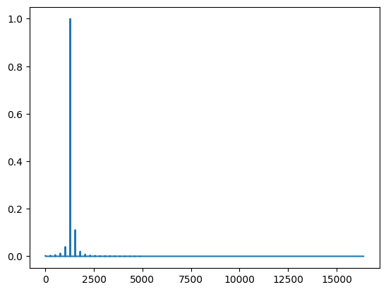
[8]:
plt.plot(tfp_data_power[:16384])
plt.show()
[9]:
# Easier to check using dB scale
tfp_data_power[tfp_data_power < 1e-10] = 1e-10

# relative power in dB
tfp_data_db = 10.0 * np.log10(tfp_data_power)
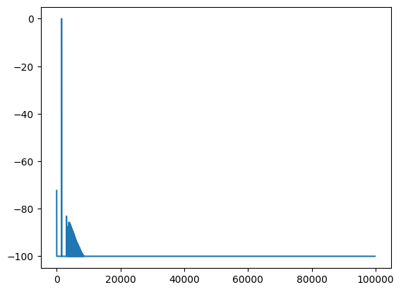
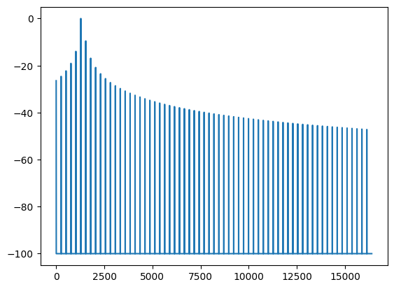
[10]:
plt.plot(tfp_data_db[:16384])
plt.show()
Use the PyDADA analyse_pfb_temporal_fidelity function to do analysis
The following cells show how to use analyse_pfb_temporal_fidelity to do the analysis and to easily check if the file passes the SKA PFB inversion requirements
[11]:
expected_to_pass: TemporalFidelityResult = analyse_pfb_temporal_fidelity(
    "data/temporal_fidelity_pass.dada",
    nifft=NIFFT,
    env_slope_db=SKA_LOW_M,
    env_halfwidth_us=SKA_LOW_W,
    max_db_outside_env=SKA_LOW_X_MAX,
    max_spurious_power_db=SKA_LOW_S_MAX,
    num_impulses=2,
    expected_impulses=[1536, 173664],
)
The output of the result can be printed as follows.
In the case of this file one can see that the overall_result is True (i.e. valid) and for each impulse there is a result which both have the following:
the impulse and the expected impulse are at the same temporal index
the
max_power_resultisTrue(i.e. valid)the
total_spurious_power_resultisTrue(i.e. valid)the
total_spurious_power_dbis <= -60 dB
[12]:
pprint.pprint(expected_to_pass)
TemporalFidelityResult(tsamp=1.08,
                       overall_result=True,
                       impulse_results=[TemporalFidelityImpulseResult(impulse_idx=1536,
                                                                      expected_impulse_idx=1536,
                                                                      valid_impulse_position=True,
                                                                      max_power_result=True,
                                                                      total_spurious_power_result=True,
                                                                      total_spurious_power_db=-70.8338212966919,
                                                                      overall_result=True),
                                        TemporalFidelityImpulseResult(impulse_idx=173664,
                                                                      expected_impulse_idx=173664,
                                                                      valid_impulse_position=True,
                                                                      max_power_result=True,
                                                                      total_spurious_power_result=True,
                                                                      total_spurious_power_db=-68.41764450073242,
                                                                      overall_result=True)])
Perform the assertions to ensure that we have the correct impulse index and assert max temporal leakage and total spurious leakage
[13]:
expected_impulses = [1536, 173664]

assert expected_to_pass.overall_result, "expected file to pass temporal fidelity analysis"

for expected_impulse_idx, r in zip(expected_impulses, expected_to_pass.impulse_results):
    assert r.expected_impulse_idx == expected_impulse_idx
    assert r.impulse_idx == expected_impulse_idx
    assert r.valid_impulse_position
    assert r.max_power_result
    assert len(r.max_power_result_idx) == 0
    assert r.total_spurious_power_result
    assert r.total_spurious_power_db <= SKA_LOW_S_MAX
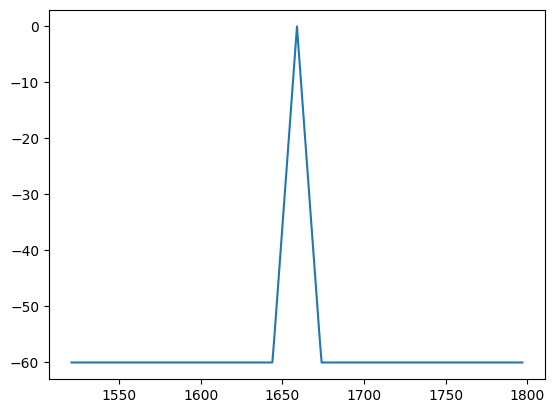
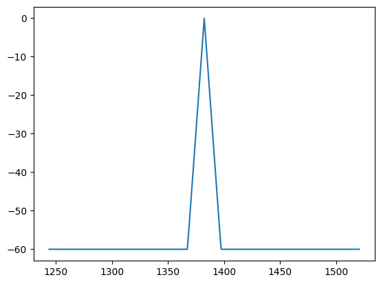
The TemporalFidelityImpulseResult has some extra attributes that can be used to show what it has calculated.
The following cells shows the maximum expected power masks for the 2 different impulses (trimmed to +-128 time samples from the impulse)
[14]:
expected_max_power_db = expected_to_pass.impulse_results[0].expected_max_power_db
max_idx = expected_to_pass.impulse_results[0].expected_impulse_idx
idx_range = np.arange(max_idx - 128, max_idx + 128 + 1)
time = expected_to_pass.tsamp * idx_range

plt.plot(time, expected_max_power_db[idx_range])
plt.show()
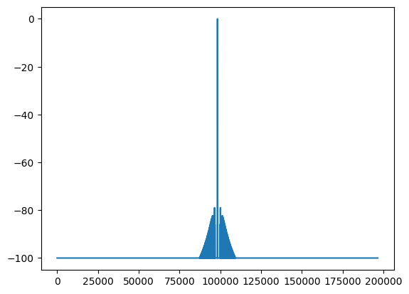
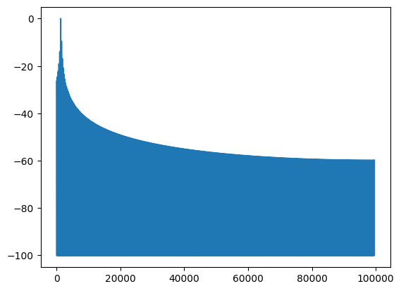
[15]:
plt.plot(expected_to_pass.impulse_results[0].signal_power_db)
plt.show()
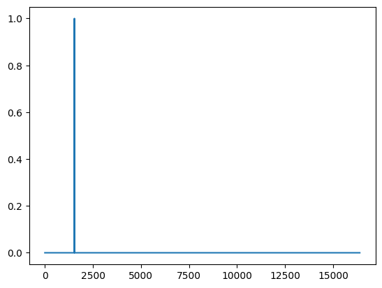
The following plot shows the same data as the manual analysis
[16]:
plt.plot(expected_to_pass.impulse_results[0].signal_power_db[:16384])
plt.show()

Plot the second impulse
[17]:
plt.plot(expected_to_pass.impulse_results[1].signal_power_db)
plt.show()
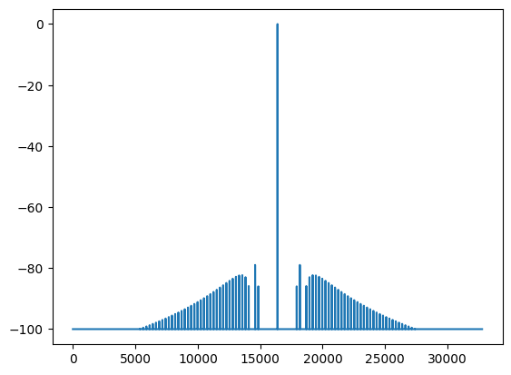
[18]:
max_id = np.argmax(expected_to_pass.impulse_results[1].signal_power_db)

plt.plot(expected_to_pass.impulse_results[1].signal_power_db[max_id - 16384 : max_id + 16384])
plt.show()
Perform analysis on a file that should fail
Inspect the DADA file data directly
In the following cells we look at the data directly without calling analyse_pfb_temporal_fidelity this can be used to visualise if there are issues
[19]:
fail_file = DadaFile.load_from_file("data/temporal_fidelity_fail.dada")
[20]:
fail_file.header
[20]:
AsciiHeader([('HDR_VERSION', '1.000000'),
             ('TELESCOPE', 'PKS'),
             ('RECEIVER', 'unknown'),
             ('SOURCE', 'TestTemporal'),
             ('MODE', 'CAL'),
             ('CALFREQ', '0.000000'),
             ('FREQ', '300.000000'),
             ('BW', '200.000000'),
             ('NCHAN', '1'),
             ('NPOL', '1'),
             ('NBIT', '32'),
             ('NDIM', '2'),
             ('STATE', 'Analytic'),
             ('TSAMP', '1.080000'),
             ('UTC_START', '2019-02-05-01:15:49'),
             ('OBS_OFFSET', '196608'),
             ('INSTRUMENT', 'dspsr'),
             ('OS_FACTOR', '4/3'),
             ('PFB_DC_CHAN', '1'),
             ('HDR_SIZE', '4096')])
[21]:
tfp_data_fail = fail_file.as_time_freq_pol().flatten()
[22]:
tfp_data_fail_power = np.abs(tfp_data_fail) ** 2.0
tfp_data_fail_power_idx = np.argmax(tfp_data_fail_power)
tfp_data_fail_power = tfp_data_fail_power / tfp_data_fail_power[np.argmax(tfp_data_fail_power)]
Plot the relative power (not in dB), it is noticeable that there seems to be some leakage
[23]:
plt.plot(tfp_data_fail_power[:16384])
plt.show()
[24]:
# Easier to check using dB scale
tfp_data_fail_power[tfp_data_fail_power < 1e-10] = 1e-10

# relative power in dB
tfp_data_fail_db = 10 * np.log10(tfp_data_fail_power)
Plotting relative power in dB shows the leakage
[25]:
plt.plot(tfp_data_fail_db[:16384])
plt.show()
Use the PyDADA analyse_pfb_temporal_fidelity function to do analysis
The following cells show how to use analyse_pfb_temporal_fidelity to do the analysis and to easily check if the file passes the SKA PFB inversion requirements
[26]:
expected_to_fail = analyse_pfb_temporal_fidelity(
    "data/temporal_fidelity_fail.dada",
    nifft=196608,
    env_slope_db=-4.0,
    env_halfwidth_us=15.0,
    max_db_outside_env=-60.0,
    max_spurious_power_db=-50.0,
    expected_impulses=[1280, 173408],
)
[27]:
pprint.pprint(expected_to_fail)
TemporalFidelityResult(tsamp=1.08,
                       overall_result=False,
                       impulse_results=[TemporalFidelityImpulseResult(impulse_idx=1280,
                                                                      expected_impulse_idx=1280,
                                                                      valid_impulse_position=True,
                                                                      max_power_result=False,
                                                                      total_spurious_power_result=False,
                                                                      total_spurious_power_db=-6.519467830657959,
                                                                      overall_result=False),
                                        TemporalFidelityImpulseResult(impulse_idx=173408,
                                                                      expected_impulse_idx=173408,
                                                                      valid_impulse_position=True,
                                                                      max_power_result=False,
                                                                      total_spurious_power_result=False,
                                                                      total_spurious_power_db=-6.317607760429382,
                                                                      overall_result=False)])
Perform the assertions to ensure that we have the correct impulse index and assert max temporal leakage and total spurious leakage
In this case we will need to assert that max temporal leakage and total spurious power fail as the file itself was set up to fail
[28]:
expected_impulses = [1280, 173408]

assert not expected_to_fail.overall_result, "expected file to fail temporal fidelity analysis"

for expected_impulse_idx, r in zip(expected_impulses, expected_to_fail.impulse_results):
    assert r.expected_impulse_idx == expected_impulse_idx
    assert r.impulse_idx == expected_impulse_idx
    assert r.valid_impulse_position
    # expect some samples to exceed the max power allowed
    assert not r.max_power_result
    assert len(r.max_power_result_idx) > 0
    # expect the total spurious power to be > -50dB
    assert not r.total_spurious_power_result
    assert r.total_spurious_power_db > SKA_LOW_S_MAX
One can check to see what indices have power outside of the allowed temporal leakage
[29]:
expected_to_fail.impulse_results[0].max_power_result_idx
[29]:
array([    0,   256,   512,   768,  1024,  1536,  1792,  2048,  2304,
        2560,  2816,  3072,  3328,  3584,  3840,  4096,  4352,  4608,
        4864,  5120,  5376,  5632,  5888,  6144,  6400,  6656,  6912,
        7168,  7424,  7680,  7936,  8192,  8448,  8704,  8960,  9216,
        9472,  9728,  9984, 10240, 10496, 10752, 11008, 11264, 11520,
       11776, 12032, 12288, 12544, 12800, 13056, 13312, 13568, 13824,
       14080, 14336, 14592, 14848, 15104, 15360, 15616, 15872, 16128,
       16384, 16640, 16896, 17152, 17408, 17664, 17920, 18176, 18432,
       18688, 18944, 19200, 19456, 19712, 19968, 20224, 20480, 20736,
       20992, 21248, 21504, 21760, 22016, 22272, 22528, 22784, 23040,
       23296, 23552, 23808, 24064, 24320, 24576, 24832, 25088, 25344,
       25600, 25856, 26112, 26368, 26624, 26880, 27136, 27392, 27648,
       27904, 28160, 28416, 28672, 28928, 29184, 29440, 29696, 29952,
       30208, 30464, 30720, 30976, 31232, 31488, 31744, 32000, 32256,
       32512, 32768, 33024, 33280, 33536, 33792, 34048, 34304, 34560,
       34816, 35072, 35328, 35584, 35840, 36096, 36352, 36608, 36864,
       37120, 37376, 37632, 37888, 38144, 38400, 38656, 38912, 39168,
       39424, 39680, 39936, 40192, 40448, 40704, 40960, 41216, 41472,
       41728, 41984, 42240, 42496, 42752, 43008, 43264, 43520, 43776,
       44032, 44288, 44544, 44800, 45056, 45312, 45568, 45824, 46080,
       46336, 46592, 46848, 47104, 47360, 47616, 47872, 48128, 48384,
       48640, 48896, 49152, 49408, 49664, 49920, 50176, 50432, 50688,
       50944, 51200, 51456, 51712, 51968, 52224, 52480, 52736, 52992,
       53248, 53504, 53760, 54016, 54272, 54528, 54784, 55040, 55296,
       55552, 55808, 56064, 56320, 56576, 56832, 57088, 57344, 57600,
       57856, 58112, 58368, 58624, 58880, 59136, 59392, 59648, 59904,
       60160, 60416, 60672, 60928, 61184, 61440, 61696, 61952, 62208,
       62464, 62720, 62976, 63232, 63488, 63744, 64000, 64256, 64512,
       64768, 65024, 65280, 65536, 65792, 66048, 66304, 66560, 66816,
       67072, 67328, 67584, 67840, 68096, 68352, 68608, 68864, 69120,
       69376, 69632, 69888, 70144, 70400, 70656, 70912, 71168, 71424,
       71680, 71936, 72192, 72448, 72704, 72960, 73216, 73472, 73728,
       73984, 74240, 74496, 74752, 75008, 75264, 75520, 75776, 76032,
       76288, 76544, 76800, 77056, 77312, 77568, 77824, 78080, 78336,
       78592, 78848, 79104, 79360, 79616, 79872, 80128, 80384, 80640,
       80896, 81152, 81408, 81664, 81920, 82176, 82432, 82688, 82944,
       83200, 83456, 83712, 83968, 84224, 84480, 84736, 84992, 85248,
       85504, 85760, 86016, 86272, 86528, 86784, 87040, 87296, 87552,
       87808, 88064, 88320, 88576, 88832, 89088, 89344, 89600, 89856,
       90112, 90368, 90624, 90880, 91136, 91392, 91648, 91904, 92160,
       92416, 92672, 92928, 93184, 93440, 93696, 93952, 94208, 94464,
       94720, 94976, 95232, 95488, 95744, 96000, 96256, 96512, 96768,
       97024, 97280, 97536, 97792, 98048, 98304, 98560, 98816, 99072,
       99328, 99584])
[30]:
expected_max_power_db = expected_to_fail.impulse_results[0].expected_max_power_db
max_idx = expected_to_fail.impulse_results[0].expected_impulse_idx
idx_range = np.arange(max_idx - 128, max_idx + 128 + 1)
time = expected_to_fail.tsamp * idx_range

plt.plot(time, expected_max_power_db[idx_range])
plt.show()
[31]:
plt.plot(expected_to_fail.impulse_results[0].signal_power_db)
plt.show()
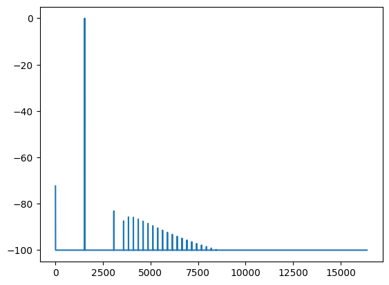
The following plot is the same from the above manual analysis
[32]:
plt.plot(expected_to_fail.impulse_results[0].signal_power_db[:16384])
plt.show()

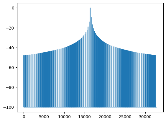
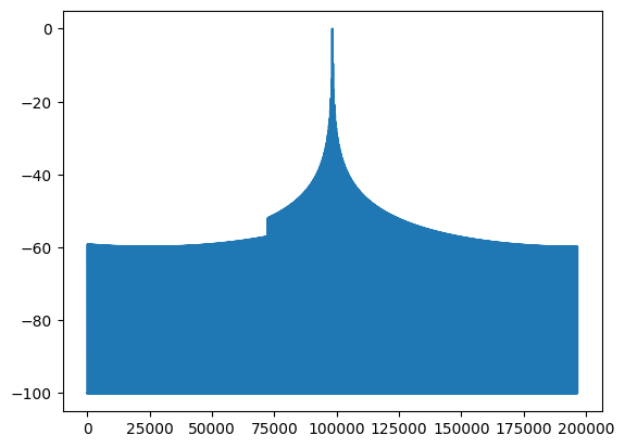
View the 2nd impulse. It is very noticeable from the dB plot that there are issues with the signal
[33]:
plt.plot(expected_to_fail.impulse_results[1].signal_power_db)
plt.show()
[34]:
max_id = np.argmax(expected_to_fail.impulse_results[1].signal_power_db)

plt.plot(expected_to_fail.impulse_results[1].signal_power_db[max_id - 16384 : max_id + 16384])
plt.show()