Generation of Model Visibilities
Embedded Element Patterns (EEPs)
Before running calibration, the Embedded Element Pattern
(EEP) images for the log-periodic antennas need to be converted to NumPy
.npy format for efficient use during calibration. This is a one-off step
and the function convert_eep2npy() is
supplied for this purpose. Standard linux wildcards can be used to apply this
function to many EEP sets at a time, or to a single set of EEPs at a given
frequency. For example, function
get_nearest_file() can be used to return
the frequency label of the nearest set of EEPs:
from ska_low_mccs_calibration.eep import get_nearest_file
channel_id = 140
channel_bw_MHz = 400.0 / 512.0
frequency_MHz = channel_id * channel_bw_MHz
file_MHz = get_nearest_file(
    "/path/to/eeps/FEKO_AAVS3_vogel_256_elem_50ohm_*MHz_?pol.mat",
    frequency_MHz,
)
And this can be passed to
convert_eep2npy() to convert to .npy
format:
from ska_low_mccs_calibration.eep import convert_eep2npy
convert_eep2npy(
    f"/path/to/eeps/FEKO_AAVS3_vogel_256_elem_50ohm_{file_MHz}MHz_?pol.mat",
    npy_dir="/path/to/eeps/npy",
)
By defaut, convert_eep2npy() will also
reduce the numerical precision of the EEP images to numpy.complex64, however this can be controlled with parameter dtype.
Local sky models
Generation of the local sky model for skymodel=”GSM” involves the following steps. When skymodel=”Sun”, the GSM2016 predict step is skipped. If the station is rotated, this is taken into account when sampling the EEPs for each sky pixel.
Import and complex conjugate the EEPs using
load_eeps().Import the PyGDSM GSM2016 model of diffuse galactic radio emission using
gsmodel()and extract all pixels above the horizon usinggsmap_lsm().Convert the instrument, sky and EEP beam models to model visibilities via a direct 3D Fourier transform using
predict_vis(). EEPs arere-sampledat the sky model pixel centres andnormalisedby the power integral over these pixels.Calculate the position of the sun and, if it is above the horizon, estimate its brightness using
solar_lsm().Use
predict_vis()to generate model solar visibilities for the sun, assuming that it is an unpolarised point source. No EEP normalisation is required.Add the galactic and solar visibilities together to form the combined model visibilities. After initial calibration, this addition may be reset using
adjust_gsm().
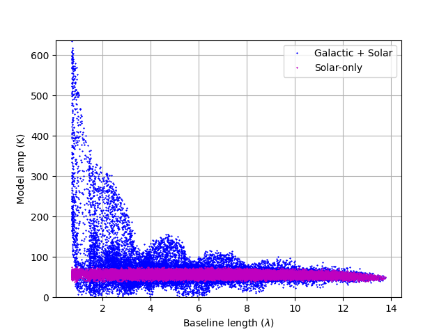
The image below shows model visibility amplitude as a function of baseline length for an AAVS3 observation with date stamp 20240119_12601 and channel ID 140 (a wavelength of 2.74m). Also shown is the contribution to the model by the sun, to highlight the galactic and solar components. These data were observed in the middle part of the day and also in the summer time when the centre of the galaxy is above the horizon during daylight hours (LST ~ 19 hours). Both components are about as strong they will be under usual conditions, and the data were readily calibrated using only a few seconds of data. However this is not a requirement. An AAVS2 dataset from a similar time of year but at night when both the sun and the centre of the galaxy were below the horizon was also well calibrated, although with a lower signal to noise ratio. This is quite promising for calibration at an arbitrary time, however care will need to be taken when generating and comparing QA metrics for different sky models, in particular metrics that involve quantities such as phase residuals that are dependent on the signal to noise level.