MID CBF MODEL
This package contains the MATLAB scripts and custom functions used for the modelling of the end-to-end signal-chain of the Square Kilometre Array (SKA) Phase-1 Correlator and Beamformer (CBF) of the Mid Telescope. This model simulates the evaluation of auto- and cross- correlations of a coherent broadband noise emitted by a point celestial source received by two or more receptors. The angular speed of the celestial source and the positions of the receptors can be set arbitrarily. Note that this model assumes an ideal receiver and an ideal analogue-to-digital convertor (ADC) [1].
Dependencies
The following Software and Toolboxes are required for the successful execution of the SKA1 Mid.CBF simulation models.
- MATLAB – Version 9.4 (or higher)
- Signal Processing Toolbox - Version 8.0 (or higher)
- Fixed-Point Designer - Version 6.1 (or higher)
Recommended System Configuration
It is recommended to have the following system configuration for efficient execution of the simulation.
Operating Systems
Windows 10
Windows 7 Service Pack 1
Processors
Minimum: Any Intel or AMD x86-64 processor
Recommended: Any Intel or AMD x86-64 processor with four logical cores and AVX2 instruction set support
Storage Space (Disk)
Minimum: 100 GB or more of HDD space as for some simulations the fine-channel time series data are saved for subsequent analysis.
RAM
Minimum: 64 GB
Recommended: 128 GB
Graphics
No specific graphics processor is required for these simulations.
References
- T. Gunaratne, SKA1 CSP Mid Correlator and Beamformer Sub-element Signal Processing MATLAB Model (EB-7) Rev 04, 311-000000-007, 2018-08-16.
Imaging Correlation Signal Chain
The signal flow graph for the imaging correlation end-to-end simulation of the SKA1 Mid.CBF is shown in Fig. 1. These simulations consider two signal paths. In the ‘unquantized’-path, unquantized signals are processed with signal processing algorithms using unquantized coefficients and the algorithms are implemented according to double-precision floating point format. In the ‘quantized’-path, quantized signals are processed with signal processing algorithms using quantized coefficients and the algorithms are implemented according to double-precision floating point format and subsequently the results are ‘requantized’. The signal processing blocks that requantized the results are shaded in gray.
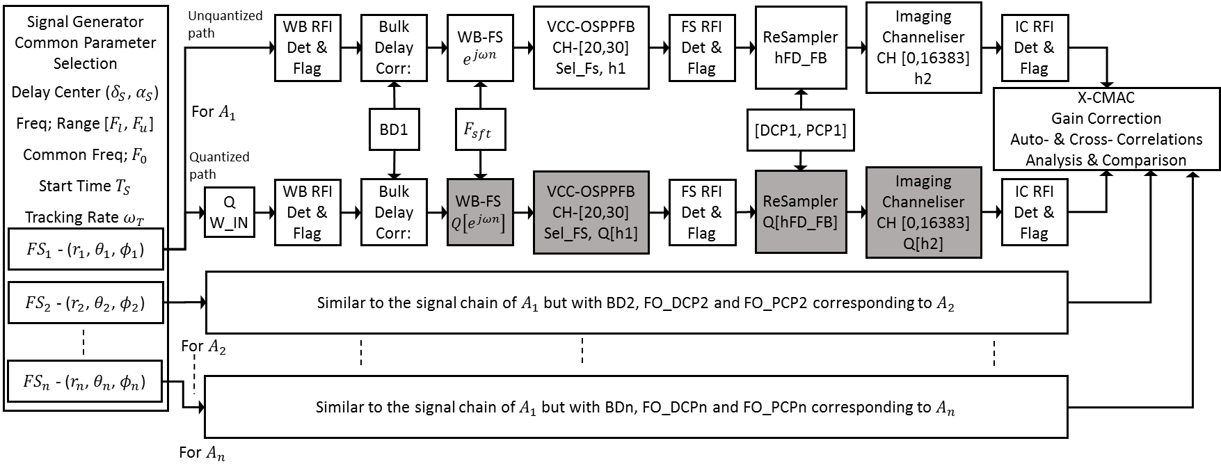
Fig. 1 Signal flow diagram of the end-to-end realizable model for the normal imaging signal chain of Mid.CBF
Signal Chain Demonstration for Imaging Correlation
The MATLAB script ‘Imaging_Demo.m’ performs a simulation of the imaging correlation of the Mid.CBF. The diagram shown in Fig. 2 illustrates the main components of the signal processing chain of the simulation. Here two signal sequences; the first corresponding to the reference receptor and the other corresponding an arbitrary receptor.
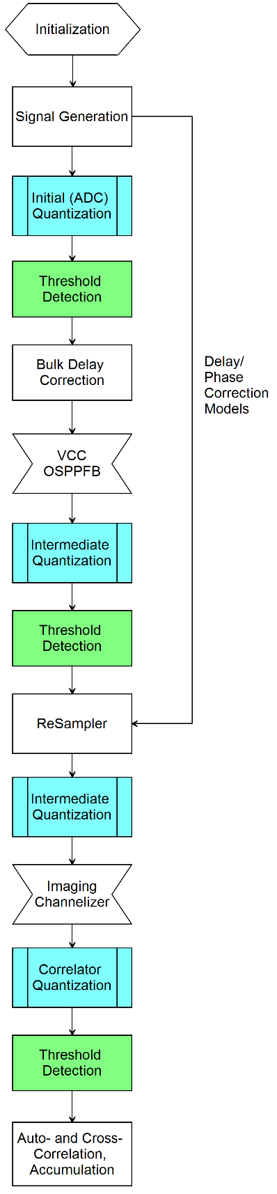
Fig. 2 The signal flow and modules of the simulator for the imaging correlation model for Mid.CBF.
The simulation is composed of a parameter specification block, followed by some signal generation discussed in Section 4.2 and signal processing steps outlined in Section 5 of [1]. First, a segment of input sequence is generated using an efficient implementation of ‘Sum of Sinusoidal’ method (Section 4.2.3 [1]). Then, these sequences are processed by the signal processing blocks shown in Fig. 2. As given in Section 4.2.2 [1], the input sequences are overlapped in simulation time in order to fill the signal processing pipeline in full. As a result, each segment of output contains invalid time samples and these are excluded from the signal analysis.
Parameter Specifications
Before running the simulation, all the parameters for the particular signal chain has to be properly initialized. Some parameters are chosen by the user. A part of the remaining parameters are selected according to the user selections and the rest are fixed. The user specified parameters for imaging simulations are listed in Table 1.
Table 1 User specified configuration parameters for imaging simulations.
| Parameter | Description |
|---|---|
| Ns_O | Number of wideband Samples in the simulation |
| Band_ID | Band Index (1, 2, 3, 4, 5 = 5a and 6=5b) |
| FS_ID | Frequency Slice Index |
| Ad_B5_Fsft | |
| WB_Fsft | Wideband Frequency Shift – in Hz |
| F_off | Frequency offset in aligning Fine channels across FSs – in Hz |
| T_si | Simulation start time – in s |
| p | Intended Correlation Coefficient (see Section 4.2.5 pp. 54) |
| F_Int | Frequency of a narrowband interferer (relative to base band Signal) – in Hz |
| A_Int_dB | Relative power of the interferer – in dB |
| P_Rep_Int | Pulse Repetition Interval – in s |
| P_Width | Pulse Width – Relative Measurement |
| Int_T0 | Interference Pulse Stat Time – in s |
| N_Pulse | Number of Pulses |
| {Rec; Positions} | Receptor positions in spherical coordinates (\(\begin{matrix} r_{i} & \theta_{i} & \rho_{i} \\ \end{matrix})\) |
| FO_Idx1 | Offset indices for SCFO sampling, an integer in (1, 2222) |
| Delay Centre | The Delay Centre – Declination and Right-Ascension angles |
| Source Position | The position of a wideband astronomical point source (close to delay centre) |
| {Sample Lengths} | The bit-length of the samples at various points of the signal chain |
| {Signal rms} | The rms levels of the signals at various points of the signal chain |
| {Threshold Detection Parameters} | Short-Temp Epoch for Power Calculation (STL) and Forgetting Factor for Long Term Power Sum (C) |
The user specified parameter ’Band_ID’ primarily set other parameters. In particular;
If Band_ID = 3, the Up-sampler is added to the signal chain after the Bulk Delay Correction.
- For Band_ID = {1, 2, 3} 20-Channel VCC-OSPPFB is selected and for Band_ID = {4, 5, 6}30-Channel VCC-OSPPFB is selected.
Other parameters are mainly fixed.
- LUT-based NCO of resolution \({\pi \bullet 2}^{- 17}\).
- ReSampler with fractional-delay filter-bank having 1024 delay-steps.
- Critically-Sampled channelizer of 16,384 channel outputs
There are other secondary parameters are specified for generation of geometric delay, evaluation of first-order delay/phase correction polynomials. It is recommended that users do not change these parameters unless there are fully aware of the functionality of the simulation model.
Test Sequence Generation
The test sequence generation procedure for the simulations are given in Section 4.2 [1]. As illustrated in Fig. 4, first, the geometrical delay vector ‘TVD_Vec’ for all receptors are evaluated using the custom MATLAB function Geomatrical_Delay_Est.m depending on the position of each receptor and the position of the source. Within the same function the first order delay and phase correction register-values (see Section 4.3.2.2.1 [1]) are generated considering the receptor locations and the delay centre. After that, the MATLAB function Rand_Seq_TVD_ChirpZ.m is used generates the pseudo-random sequence ‘s_Vec’, using an efficient implementation of Sum-of-Sinusoid method using the chirp-z algorithm. For each receptor, the corresponding sequence in s_Vec’ that associates the corresponding delay in ‘TVD_Vec’ is sampled at the sample times ‘ST_Vec’. Note that the spectrum of ‘s_Vec’ is flat within the observation band.
The signal ‘s_Vec’, which mimics the wideband astronomical signal, is then combined with two other signals, representing respectively the band-limited uncorrelated receiver (and sky) Gaussian noise ‘n_Vec’, and a Gaussian pulse-train representing time varying RFI ‘int_Vec’, to synthesize the ‘received’ Receptor signal sequence ‘x_Vec’. The receiver noise is generated using the custom MATLAB function ‘Gaussian_Noise.m’. It also has a flat spectrum in the receiver bandwidth, and it is scaled to achieve a certain correlation coefficient ‘p’ for the ‘s_Vec’. The MATLAB function ‘pulstran.m’ is used to generate a ‘Gaussian’ pulse train mimicking an RFI signal. This function generates a set of ‘N_Pulse’ pulses at frequency specified by the ‘F_Int’, with an amplitude (in dB) defined by ‘Int_Scale’ sampled at times ‘ST_Vec’.
Quantization Blocks
As shown in Fig. 3, the quantization stage shown is preceded by a scaling block. In the first iteration of the simulation, the signal level is examined by the scaling block, determining the appropriate scaling according to the user specified level (e.g. ‘Peak_to_IP_RMS_Ratio’), and is applied to all subsequent iterations. After scaling the quantization is performed using the MATLAB ‘sfi.m’ function. Finally, the quantized signal is rescaled to achieve the same signal level as the un-quantized signal.
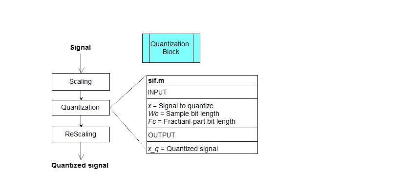
Fig. 3 The signal quantization block.
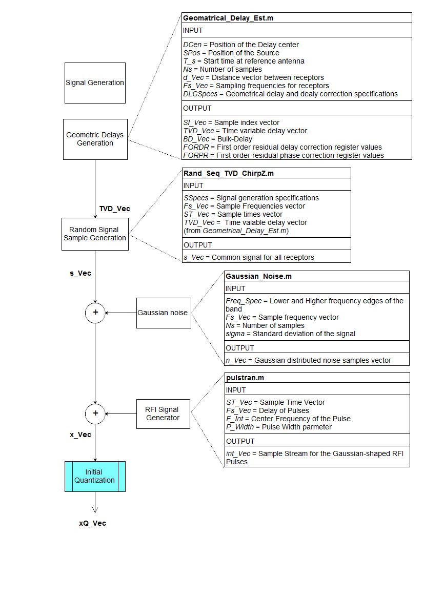
Fig. 4 Test sequence generation for imaging simulation.
Threshold Detection
The custom MATLAB function ‘Threshold_Det.m’, shown in Fig. 4 is used to detect and flag potential RFI. The detection is based on the increase in the instantaneous power in the presence of strong RFI in ‘x_Vec’ or ‘xQ_Vec’. The instantaneous ‘Short-Term’ power is calculated for a moving-window of programmable length ‘STAL’. If the instantaneous power exceeds the specified threshold-level ‘STPTL’, a flag is to the current sample. Also, in order to facilitate optimum scaling before re-quantization, the ‘Long-Term’ power is calculated through integration using “Backward Euler Method” without considering the flagged’ samples.
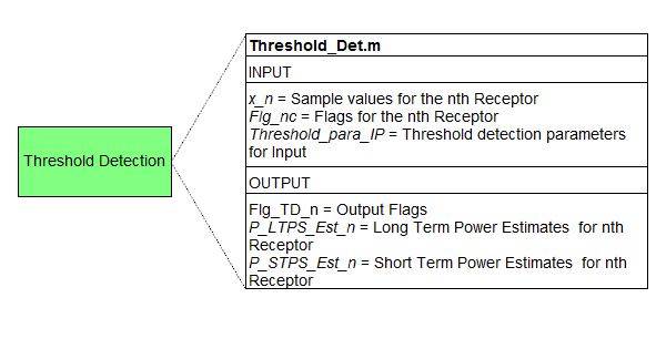
Fig. 5 The Threshold Detection Block
Imaging Signal Chain
For all Bands except Band 3, the vector of input sequences ‘x_Vec’ are processed by VCC-OSPPFB. For Band 3, ‘x_Vec’ are first processed by an ‘up-Sampler’ (see Section 4.3.3 [1]) and then processed by VCC-OSPPFB. Here, only one FS is extracted using the model of VCC-OSPPFB. The extracted FS is corrected for delay, sampling frequency offset and phase, and is channelized again in to fine channels using the imaging channelizer. Signals from all receptors are processed in parallel.
The custom MATLAB function ‘OS_Poly_DFT_FB_SC.m’, shown in Fig. 6, models an over-sampled Polyphase DFT Filter-Bank (OSPPFB) and yields the time-series samples for the selected FS. Note that FSs corresponding to different receptors are at different sample rates.
There is A ‘Threshold Detection’ block after the VCC-OSPPFB to detect RFI that is associated with non-linear components or that could generate non-linear components in the subsequent signal processing stages. The custom MATLAB function ‘Threshold_Det.m’ with the appropriate patrameters performs this function.
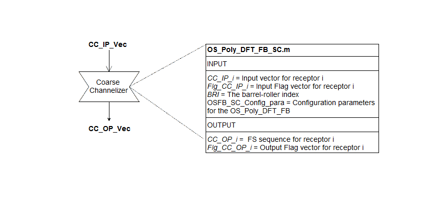
Fig. 6 The VCC-OSPPFB module.
Then, the FS are resampled using fractional-delay filter banks and phase-corrected with phase-rotators in order to correct the delay and phase with respect to the delay-centre at boresight and resample the SCFO sampled sequences. As shown in Fig. 7, the resampling process is modelled by the custom MATLAB function ‘ReSampler_ERP_Corr.m’.
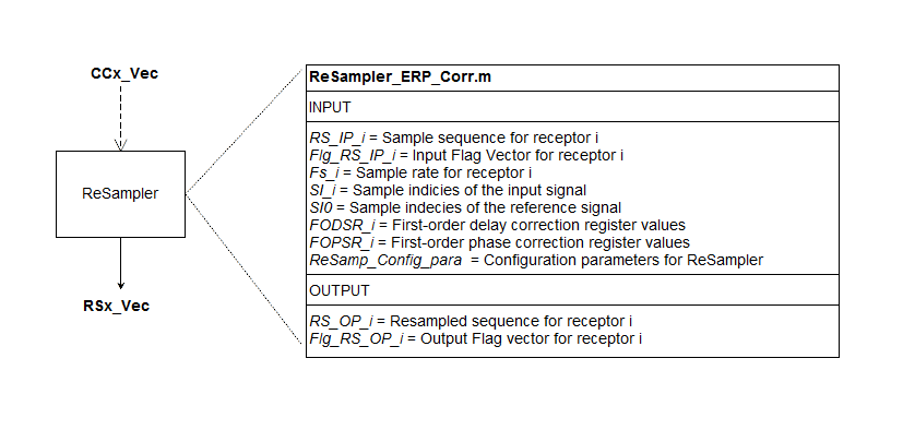
Fig. 7 The ReSampler module for delay/phase correction.
The resampled signals are then processed by the Imaging Channelizer, a critically-sampled polyphase DFT filter bank, producing 16,384 channels. This is modelled by the custom MATLAB function ‘CS_Poly_DFT_FB_Batch.m’, shown in Fig. 8.
The imaging channels are subjected to gain corrections to compensate the passband ripple effect due to the preceding signal processing modules. Then, each imaging channel is analysed for RFI using ‘Threshold_Det_NCh.m’. Note that ‘Threshold_Det_NCh.m’ and ‘Threshold_Det.m’ are almost identical except that ‘Threshold_Det_NCh.m’ is capable of applying the flagging for a programmable window.
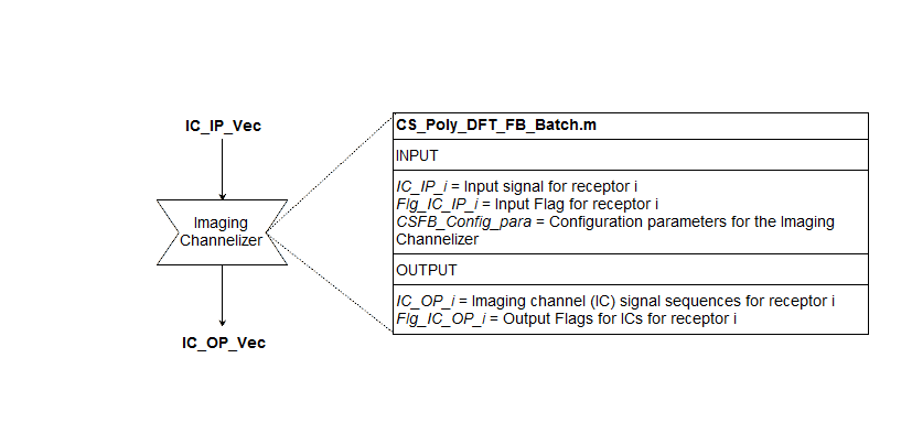
Fig. 8 The Imaging Channelizer module.
After the gain corrections, the pairs of imaging channels are cross multiplies and accumulated to evaluate the auto- and cross- correlations.
Results
In the ‘Imaging_Demo.m’ the objective is to have an understanding of the changes of the signal characteristics along the signal chain. Here, all intermediate data products are retained. Therefore, post processing analysis can be performed on any input and output combinations. Also, Set of figures are generated as the simulation progress along the signal chain.
Simulations for Generating Integrations of Specific Duration
In order to evaluate auto- and cross- correlations for a specific duration (i.e. 10 ms to 10 sec), the above sequence is iterated several times. Note that the signal generation process is highly memory intensive and therefore, with the available resources it can only generate wideband signals spanning few milliseconds.
The MATLAB script ‘Imaging_Running_Simulation_NRecps.m’ performs the iterative evaluation of auto and cross correlations for a duration if ‘T_Sim’ combining signals from ‘N_Rcp’ number of receptors. In these simulations, no intermediate data products are saved except for the imaging channels after ripple corrections.
| [1] | There is related model that has been developed that combines a model for the SKA1 Dish receiver and digitizer and the model for SKA1 Mid.CBF. That is expected to release later in collaboration with the developer of that model. |